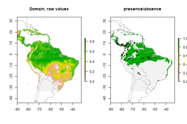
Thresholding species distribution models

Apr 12, 2019 5 min read R, species distribution modeling

From left to right: unmodified species distribution model, minimum training presence threshold, and 10th percentile threshold.

Inspiration for this post

Conservation is often the main motivation behind studying where a species lives – having a model of a species’ range can help scientists assess whether it is at risk of extinction, designate protected regions to preserve its habitat, and study potential impacts of human activity. When we create species distribution models using common methods like Maxent, the result is a map of predicted habitat suitability or probability of species presence, such as the one below. In conservation management, however, it is often more useful to present range models in the form of species presence/absence. We can convert continuous predictions of habitat suitability into binary predictions of whether a species lives in a certain region or not using thresholds: i.e. designating all regions above a certain suitability level as within the species range and all areas below that suitability level as outside of it.

Left: species distribution model with continuous habitat suitability values. Right: binary presence/absence model used by applying a threshold. (Figure from Spatial Data Science with R)

I recently needed to threshold some species distribution models to convert them into these binary maps and had difficulty finding a built-in way to do this in R. The dismo package for species distribution modeling has a function threshold to find what value to use as the “cut-off”, but I needed a function to apply a given cut-off value to model and output a raster with binary values for presence and absence.

Thresholding function

I wrote an R function to take a species distribution model and threshold it by a given threshold - either minimum training presence (MTP) or 10th percentile training present (P10).

Minimum training presence

This threshold finds the lowest predicted suitability value for an occurrence point. Essentially, it assumes that the least suitable habitat at which the species is known to occur is the minimum suitability value for the species. The MTP threshold ensures that all occurrence points fall within the area of the binary model.

10th percentile training presence

The P10, on the other hand, is a threshold which omits all regions with habitat suitability lower than the suitability values for the lowest 10% of occurrence records. It assumes that the 10% of occurrence records in the least suitable habitat aren’t occurring in regions that are representative of the species overall habitat, and thus should be omitted. This threshold omits a greater region than the MTP.

The function

The following is the function I wrote to apply these two thresholds to an SDM. The function’s arguments are the SDM, the occurrence points of the species in the form of longitude - latitude pairs, the threshold type, and whether the user would like the output to be a binary prediction (0s for predicted absence and 1s for predicted presence), or a thresholded continuous SDM (regions with suitability below the threshold set to 0).

library(raster)
## Loading required package: sp


sdm_threshold <- function(sdm, occs, type = "mtp", binary = FALSE){
  occPredVals <- raster::extract(sdm, occs)
  if(type == "mtp"){
    thresh <- min(na.omit(occPredVals))
  } else if(type == "p10"){
    if(length(occPredVals) < 10){
      p10 <- floor(length(occPredVals) * 0.9)
    } else {
      p10 <- ceiling(length(occPredVals) * 0.9)
    }
    thresh <- rev(sort(occPredVals))[p10]
  }
  sdm_thresh <- sdm
  sdm_thresh[sdm_thresh < thresh] <- NA
  if(binary){
    sdm_thresh[sdm_thresh >= thresh] <- 1
  }
  return(sdm_thresh)
}

The first step of the function is to extract the SDM predictions at all occurrence points.

occPredVals <- raster::extract(sdm, occs)

Next, the function calculates a threshold value thresh for either the MTP or P10 threshold. Finally, it sets all cells in the SDM raster with values lower than the threshold equal to 0. If the user wants a binary map, the function sets all cells above the threshold equal to 1:

sdm_thresh <- sdm
sdm_thresh[sdm_thresh < thresh] <- NA
if(binary){
  sdm_thresh[sdm_thresh >= thresh] <- 1
}

Example

Now we can apply the function to an actual SDM I generated for a species of three-toed sloth (Bradypus variegatus).

# load in the SDM and occurrence points
sloth_sdm <- raster("../../../static/SDMs/variegatus_sdm.tif")
sloth_occs <- read.csv("../../../static/SDMs/variegatus_occ.csv")

plot(sloth_sdm)
points(sloth_occs[,2:3], pch = 19, cex = 0.5)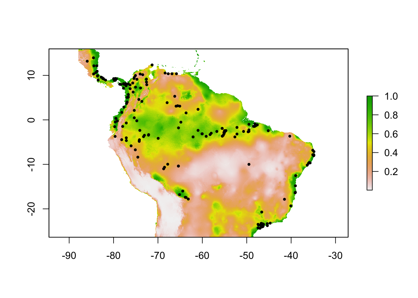

We can apply both MTP and P10 thresholds to the SDM based on the location of the occurrence points:

sloth_mtp <- sdm_threshold(sloth_sdm, sloth_occs[,2:3], "mtp")
plot(sloth_mtp)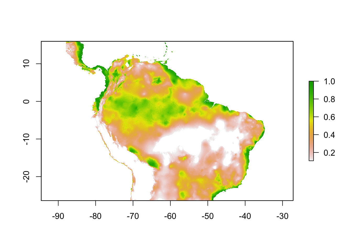


sloth_p10 <- sdm_threshold(sloth_sdm, sloth_occs[,2:3], "p10")
plot(sloth_p10)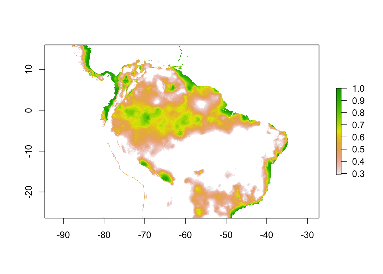

We could also make either of these thresholded SDMs into a binary prediction in the following way:

sloth_mtp_bin <- sdm_threshold(sloth_sdm, sloth_occs[,2:3], "mtp", binary = TRUE)
plot(sloth_mtp_bin)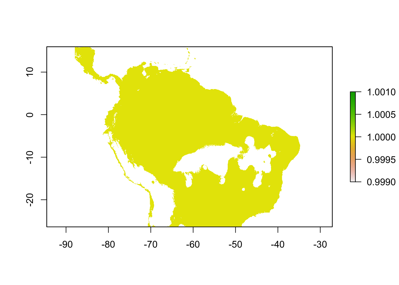

Generalization

My primary motivation to write this function was to use it on SDMs, but the function could easily be generalized to threshold any raster by a given value:

raster_threshold <- function(input_raster, points = NULL, type = NULL, threshold = NULL, binary = FALSE) {
  if (!is.null(points)) {
    pointVals <- raster::extract(input_raster, points)
    if (type == "mtp") {
      threshold <- min(na.omit(pointVals))
    } else if (type == "p10") {
      if (length(pointVals) < 10) {
        p10 <- floor(length(pointVals) * 0.9)
      } else {
        p10 <- ceiling(length(pointVals) * 0.9)
      }
      threshold <- rev(sort(pointVals))[p10]
    }
  }
  raster_thresh <- input_raster
  raster_thresh[raster_thresh < threshold] <- NA
  if (binary) {
    raster_thresh[raster_thresh >= threshold] <- 1
  }
  return(raster_thresh)
}

I expanded the function to allow the user to input points within the raster to calculate MTP and P10 thresholds if desired, but also to enable a user-specified threshold.

# create arbitrary raster
raster1 <- raster(nrow=10, ncol=10)
raster1[1:25]<- 1:25
raster1[26:50] <- rev(1:25)
raster1[51:75] <- 1:25
raster1[76:100] <- rev(1:25)

# create a set of 20 arbitrary points within the raster
xy <- data.frame(x = runif(20, min = -150, max = 150), y = runif(20, min = -70, max = 70))

plot(raster1)
points(xy)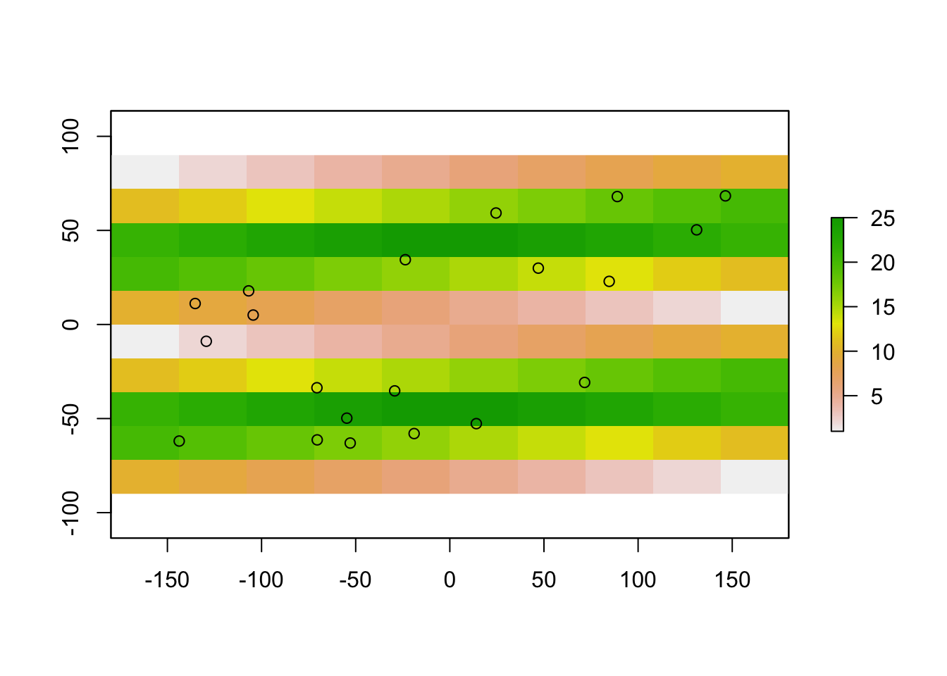

Now we can apply the function to see the MTP and P10 thresholded rasters:

mtp_raster <- raster_threshold(input_raster = raster1, points = xy, type = "mtp", binary = TRUE)
plot(mtp_raster)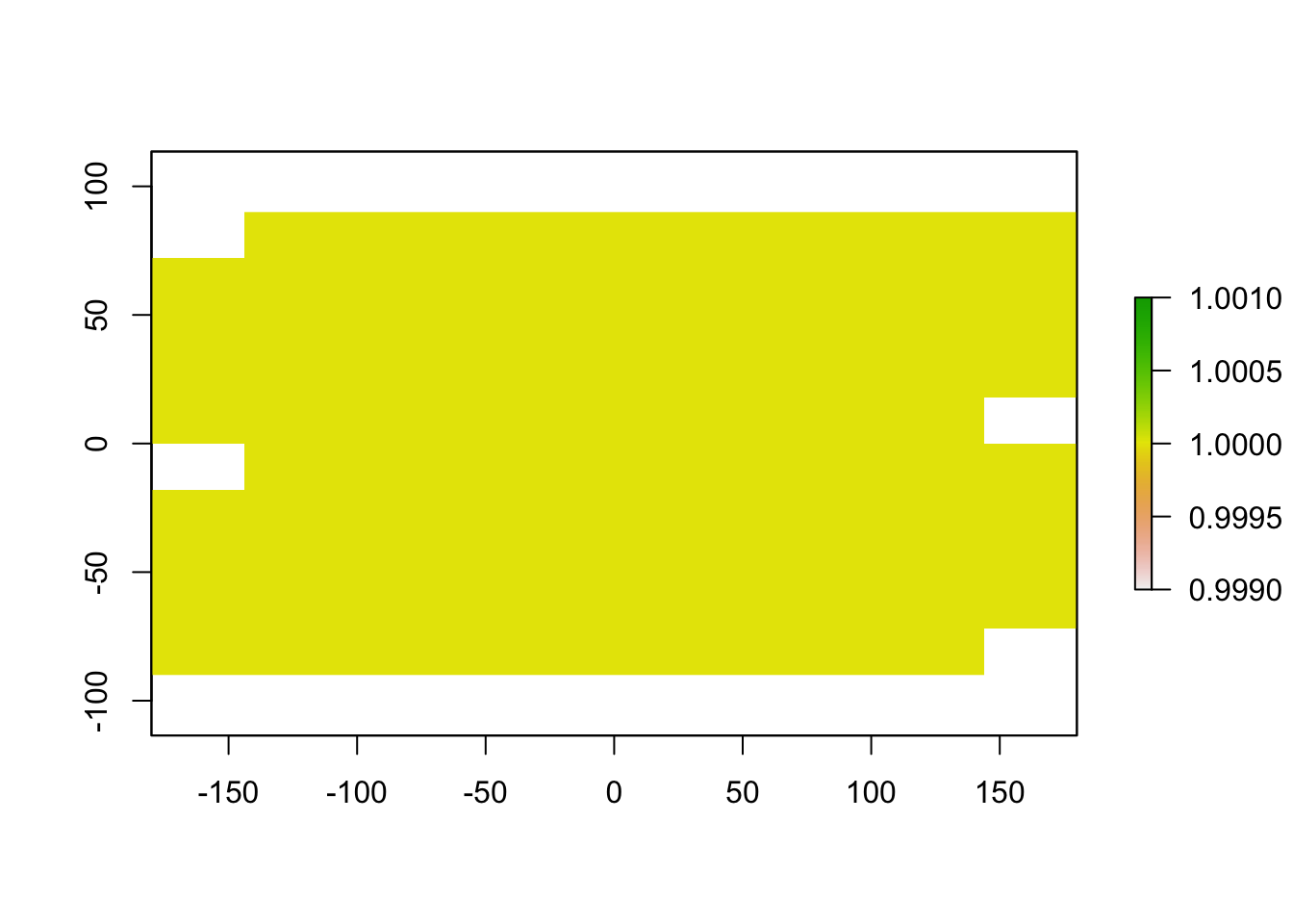


p10_raster <- raster_threshold(input_raster = raster1, points = xy, type = "p10", binary = TRUE)
plot(p10_raster)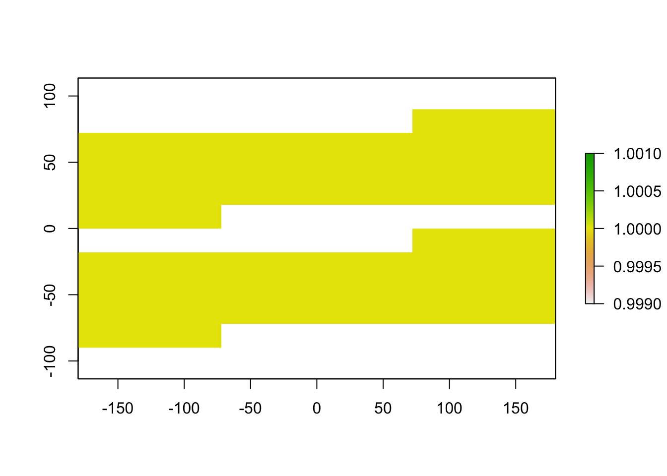

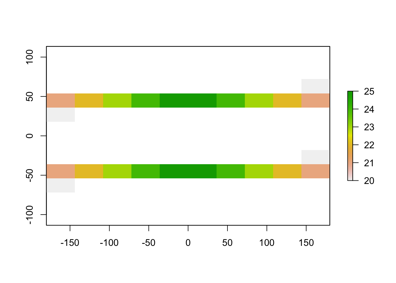
We can also use a user-inputted threshold to remove all parts of the raster with values lower than 20:

user_raster <- raster_threshold(input_raster = raster1, threshold = 20)
plot(user_raster)

R species distribution modeling