Grafting phylogenies
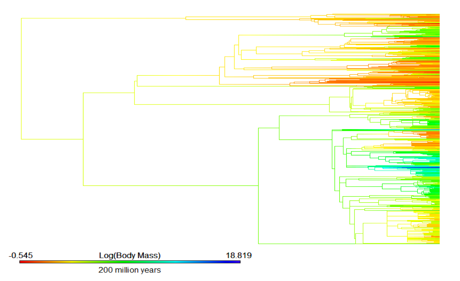
Inspiration for this post
This post comes from the finishing touches I needed to put on a paper about life history evolution. The paper compares life history traits across the four groups of tetrapods (amphibians, reptiles, mammals, and birds), so when I carried out the nitty gritty phylogenetic analyses, I used four separate phylogenies. When it came time to make a figure to visualize those analyses, however, I ended up with an unwieldy (and unpublishable) 16-panel figure (four phylogenies by four traits). One of my coauthors suggested using a tetrapod supertree to visualize the evolution of the traits across all four classes simultaneously.
Uyeda et al. 2017
Uyeda et al. did something similar in their 2017 paper The evolution of energetic scaling across the vertebrate tree of life. They stitched together fish, amphibian, squamate, bird, and mammal phylogenies together to visualize metabolic rate across all vertebrates:
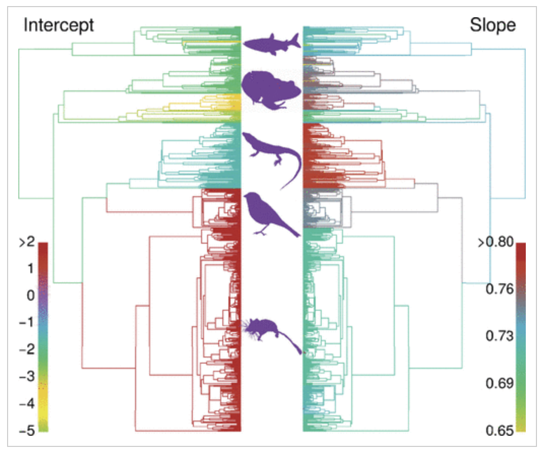
At first, I was very hopeful that I would be able to download this supertree and prune it to the taxa in my analysis since the authors were using the same clade specific phylogenies that I was. The phylogeny is available on Data Dryad (https://datadryad.org/resource/doi:10.5061/dryad.3c6d2). Unfortunately, after downloading that phylogeny and pruning it to include species I used in my analysis, I ended up with approximately 15% of the species I analyzed in the resulting tree.
Into the code
Since my easy solution didn’t pan out and I couldn’t get enough information from the supplemental material for the paper to replicate their analyses, I looked on GitHub to try to find Uyeda’s code. Hooray for GitHub once again, because the repository for the paper can be found here: https://github.com/uyedaj/bmr. The RMarkdown details the analyses for the paper, including the process for making the full tree.
Start with loading the necessary packages.
library(phytools)
## Loading required package: ape
## Loading required package: mapslibrary(geiger)The original phylogenies
I was working with four separate phylogenies: amphibians, squamates, birds, and mammals. For amphibians, I used a congruified time-tree from the PhyloOrchard package (O’Meara et al. 2013) that was constructed using the Alfaro et al. timetree of gnathostomes (Alfaro et al. 2009) as the reference and the Pyron and Wiens amphibian phylogeny as the target (Pyron and Wiens 2011).
length(amphibiantree$tip.label)
## [1] 2871
plot(amphibiantree, type = "fan", show.tip.label = FALSE)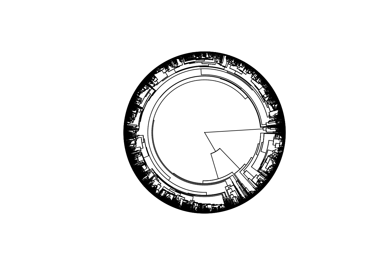
For squamates, I used the Zheng and Wiens time-calibrated phylogeny (Zheng and Wiens 2016).
length(squamatetree$tip.label)
## [1] 378
plot(squamatetree, type = "fan", show.tip.label = FALSE)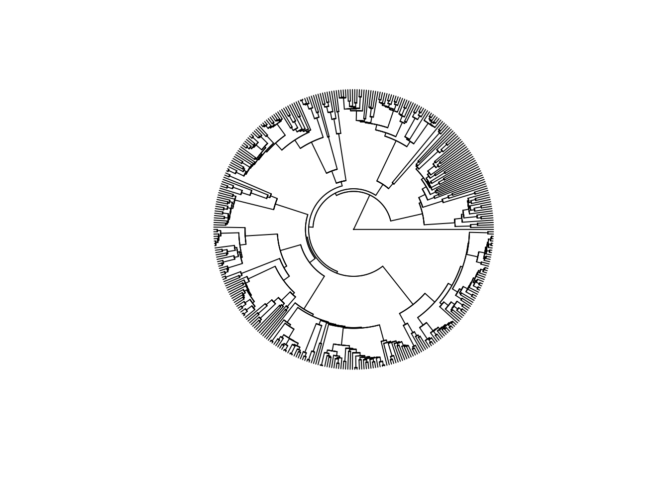
For birds, I used the Jetz phylogeny (Jetz et al. 2012).
length(birdtree$tip.label)
## [1] 9993
plot(birdtree, type = "fan", show.tip.label = FALSE)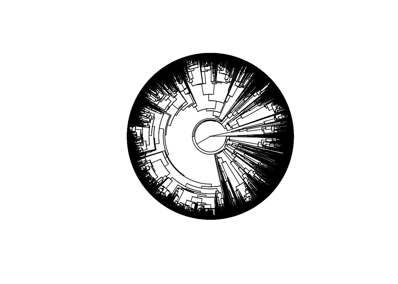
For mammals, I used the supertree from Fritz et al. 2009.
length(mammaltree$tip.label)
## [1] 5020
plot(mammaltree, type = "fan", show.tip.label = FALSE)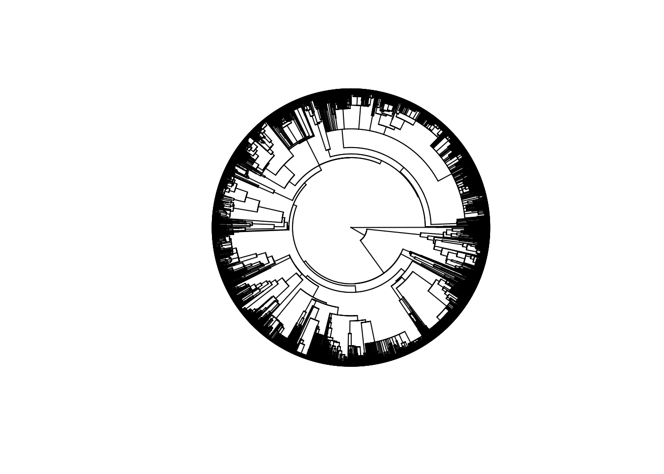
Reading in trees
The first step of the process is reading in the individual phylogenies you want to stitch together. This step is straightforward, with one exception: you cannot have species that are present in multiple of the individual trees. For example, my squamate phylogeny included Gallus gallus (red junglefowl) and Dromaius novaehollandia (emu). Since these species were also present in my bird phylogeny, I got the following error: Found matching tips in 'subtree' and 'phy'. To solve this problem, I just removed these tips from the squamate tree:
squamatetree <- drop.tip(phy = squamatetree, tip = c("Gallus_gallus", "Dromaius_novaehollandiae"))I ended up with the following list of trees and corresponding tip labels:
tree_list <- list(amphib=amphibiantree, birds=birdtree, squam=squamatetree, mamm=mammaltree)
class(tree_list) <- "multiPhylo"
Make a tree with orders
In Uyeda et al. (2017), the authors were creating a phylogeny for all vertebrates, but for my analyses I was only examining tetrapods, so I didn’t have a fish phylogeny to include. The original code from Uyeda et al. to create a tree with the 5 vertebrate orders looks like this:
tip.labels <- c("fish", "amphib", "squam", "birds", "mamm")

## Make a tree with just orders:
edge <- matrix(c(9, 4,
  9, 3,
  8, 5,
  8, 9,
  7, 8,
  7, 2,
  6, 7,
  6, 1), byrow=TRUE, ncol=2)
## Dates from Timetree of life (timetree.org)
edge.length <- c(274.9, 274.9, 324.5, 324.5-274.9, 382.9-324.5, 382.9, 454.6-382.9 , 454.6)
Nnode <- 4
ordertree <- list(edge=edge, Nnode=Nnode, tip.label=tip.labels, edge.length=edge.length)
class(ordertree) <- 'phylo'
plot(ordertree)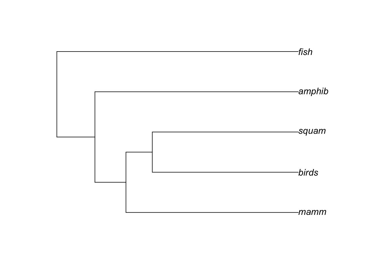
To visualize the results, we can add tip labels, node labels, and edge labels to the tree with the branch lengths:
plot(ordertree)
tiplabels()
nodelabels()
edgelabels(ordertree$edge.length, bg="black", col="white", font=2)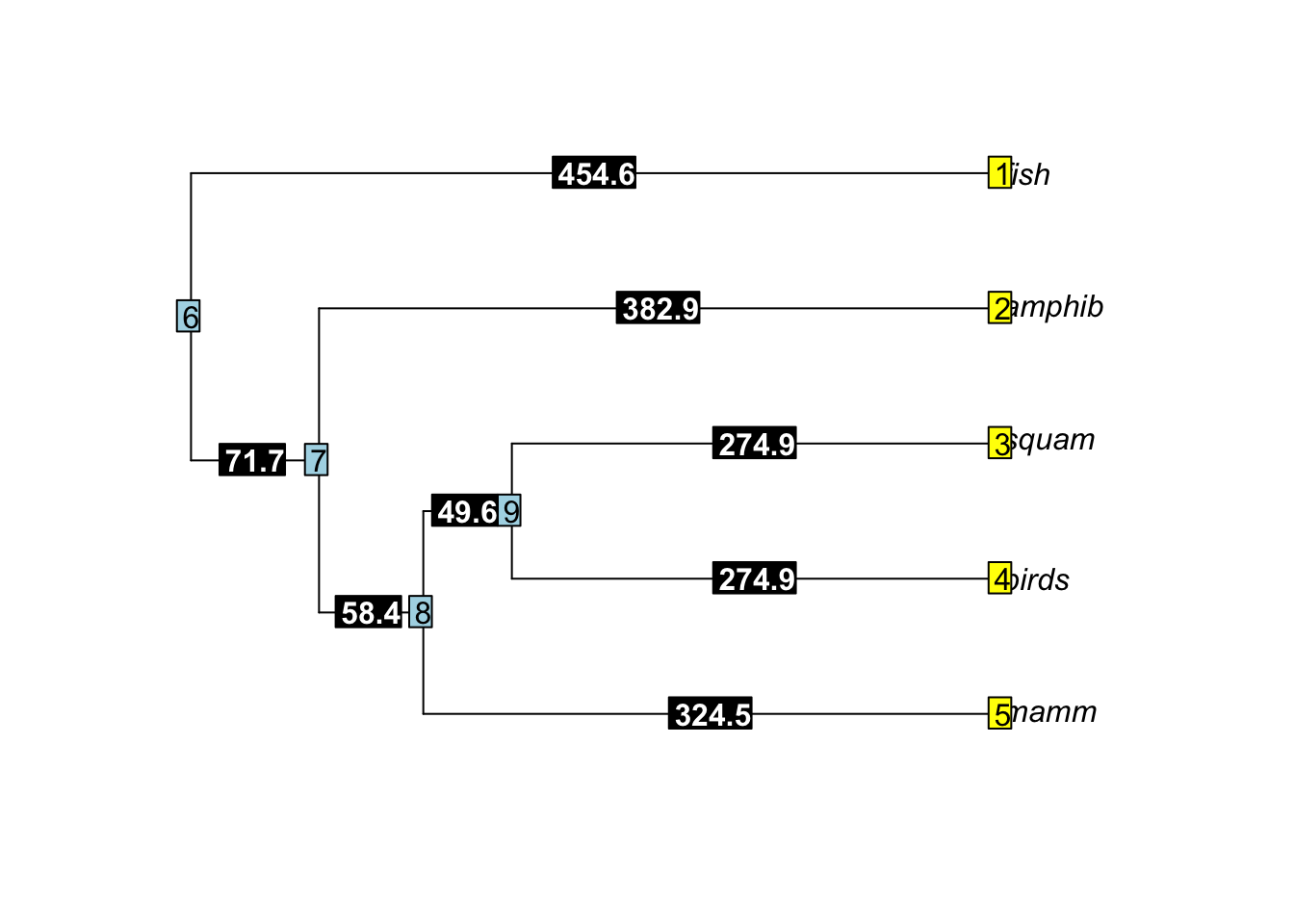
Getting rid of fish
Since I didn’t have fish, I needed to make a few modifications. First, tip.labels didn’t need “fish” in it anymore:
# remove "fish" from tip.labels:
tip.labels <- c("amphib", "squam", "birds", "mamm")
Now, for the trickier part - I needed to modify the edge matrix. The edge matrix contains the starting and ending nodes for each edge in a tree. As we can see from the plot above, numbering works in the following way: the tips are numbered starting at the top from 1 to the number of tips and the nodes are numbered starting at the root and moving towards the tips. To get rid of fish, I needed to delete one tip from the tree and one node (the original root node). I sketched out what I wanted the new order tree to look like, complete with numbered nodes and tips, and created the following edge matrix:
edge <- matrix(c(7, 3,
  7, 2,
  6, 4,
  6, 7,
  5, 6,
  5, 1), byrow=TRUE, ncol=2)
Since I was losing two edges from the phylogeny (the one going from the root to fish and the one from the root to the last common ancestor of tetrapods), I also needed to modify the edge lengths by removing 454.6-382.9 and 454.6:
edge.length <- c(274.9, 274.9, 324.5, 324.5-274.9, 382.9-324.5, 382.9)The final modification I needed was to decrease Nnode from 4 to 3:
Nnode <- 3So now…
ordertree <- list(edge=edge, Nnode=Nnode, tip.label=tip.labels, edge.length=edge.length)
class(ordertree) <- 'phylo'
plot(ordertree)
edgelabels(ordertree$edge.length, bg="black", col="white", font=2)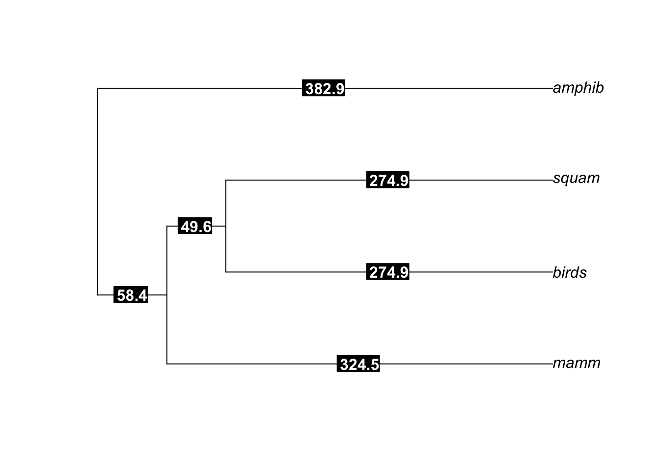
…I was ready to go with an order-level tree onto which I could graft my individual phylogenies!
Node dates
…Not so fast. I ended up with an additional problem I needed to solve before grafting the trees together. I ran into the error 'split_age' is inconsistent with edge lengths in 'phy', which means that the earliest node in one of my individual phylogenies was older than the node age I gave in edge.length. By using debug, I was able to tell that the error occurred when I added the squamate tree. The oldest node in my squamate tree was 277.8 million years ago, but I had set the divergence time between birds and squamates at 274.9 mya, so R was having problems. The species causing the problem was the tuatara, which is the only surviving member of its order.
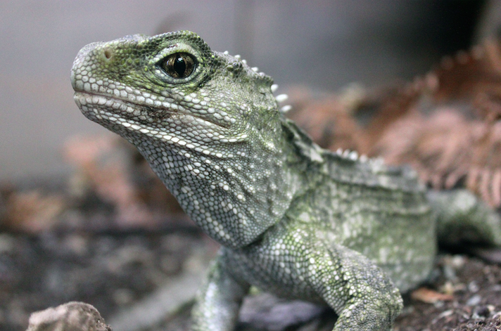
I had a couple of choices: either delete the tuatara from the squamate phylogeny or increase the age of the last common ancestor of birds and squamates when I created the vector edge.length. I chose to do the latter because why get rid of such a cool animal!
I went to http://timetree.org/ to see if I could find a reasonable range of estimates for this node. According to the website, which allows you to search for the divergence time between any two taxa, the estimated divergence of birds and squamates occurred 280 mya.
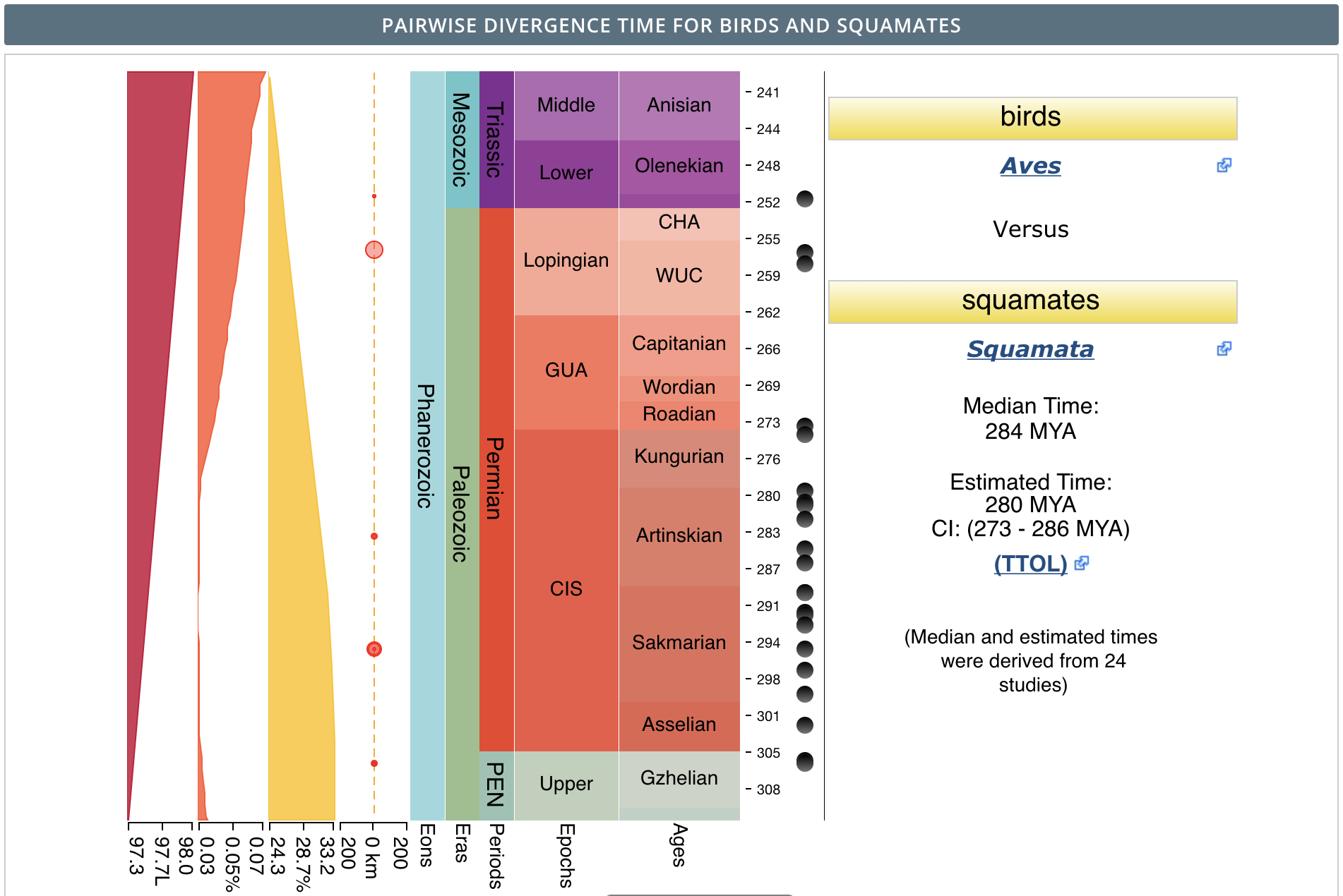
So I ended up with the following code and order tree:
tip.labels <- c("amphib", "squam", "birds", "mamm")
edge <- matrix(c(7, 3,
  7, 2,
  6, 4,
  6, 7,
  5, 6,
  5, 1), byrow=TRUE, ncol=2)
edge.length <- c(280, 280, 324.5, 324.5-274.9, 382.9-324.5, 382.9)
Nnode <- 3
ordertree <- list(edge=edge, Nnode=Nnode, tip.label=tip.labels, edge.length=edge.length)
class(ordertree) <- 'phylo'
plot(ordertree)
edgelabels(ordertree$edge.length, bg="black", col="white", font=2)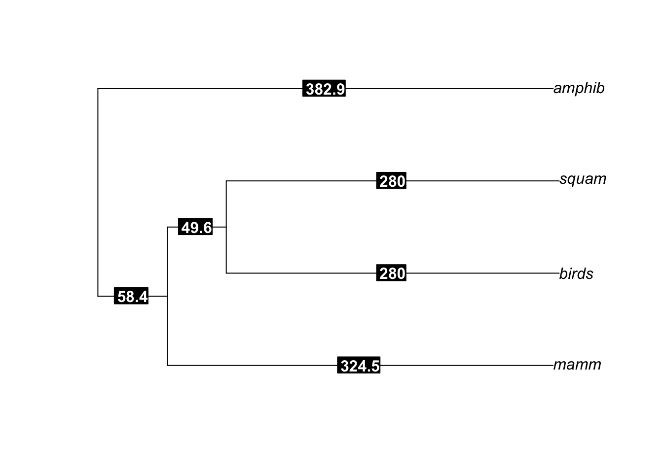
tree_list <- list(amphib=amphibiantree, birds=birdtree, squam=squamatetree, mamm=mammaltree)
class(tree_list) <- "multiPhylo"
Grafting the trees
The final step is grafting the individual trees onto the order tree in the proper place.
#Add taxonomic information to tree
otax <- data.frame("Class"= ordertree$tip.label, "Superclass"=c(rep("Tetrapoda",2)))
rownames(otax) <- ordertree$tip.label
classtree <- nodelabel.phylo(ordertree, otax, ncores=1)

res <- glomogram.phylo(classtree, tree_list)
plot(res, type = "fan", show.tip.label = FALSE)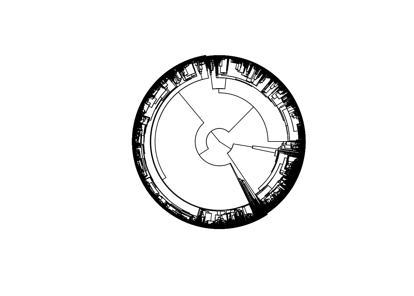
Voila - a tree with 18262 species of tetrapods!
Disclaimer
I’d like to finish this post with a disclaimer: I am NOT a phylogeneticist (yet?). The supertree created in this analysis incorporates several different phylogenies from literature and adapts code from another published article (all written by people with much more phylogenetic background than I!). However, the accuracy of the tree decreases as you move back in time - there is a great deal of uncertainty about node age for the deeper nodes in the tree. Even so, this process allows us to make some cool visualizations to compare major clades across vast stretches of evolutionary time - even if precise dates are incorrect, overall patterns are still informative!
Code
The entire script I used for this process can be found at https://github.com/KerkhoffLab/bodymasspatterns/blob/master/tetrapod_phylogeny_code.R.
#Literature Cited
Alfaro, M. E., F. Santini, C. Brock, H. Alamillo, A. Dornburg, D. L. Rabosky, G. Carnevale, and L. J. Harmon. 2009. Nine exceptional radiations plus high turnover explain species diversity in jawed vertebrates. PNAS 106:13410-13414.
Fritz, S. A., O. R. P. Bininda-Emonds, and A. Purvis. 2009. Geographical variation in predictors of mammalian extinction risk: big is bad, but only in the tropics. Ecology Letters 12:538–549.
Jetz, W., G. H. Thomas, J. B. Joy, K. Hartmann, and A. O. Mooers. 2012. The global diversity of birds in space and time. Nature 491:444.
O’Meara, B. C., L. J. Harmon, and J. Eastman. 2013. PhyloOrchard: Important and/or useful phylogenetic datasets.
Pyron, R. A. and J. J. Wiens. 2011. A large-scale phylogeny of Amphibia including over 2800 species, and a revised classification of extant frogs, salamanders, and caecilians. Molecular Phylogenetics and Evolution 61: 543-583.
Uyeda JC, Pennell MW, Miller ET, Maia R, McClain CR (2017) The evolution of energetic scaling across the vertebrate tree of life. The American Naturalist 190(2): 185-199. https://doi.org/10.1086/692326
Uyeda JC, Pennell MW, Miller ET, Maia R, McClain CR (2017) Data from: The evolution of energetic scaling across the vertebrate tree of life. Dryad Digital Repository. https://doi.org/10.5061/dryad.3c6d2
Zheng, Y., and J. J. Wiens. 2016. Combining phylogenomic and supermatrix approaches, and a time-calibrated phylogeny for squamate reptiles (lizards and snakes) based on 52 genes and 4162 species. Molecular Phylogenetics and Evolution 94:537–547.