Converting alpha hulls to spatial objects
Inspiration for this post
In species distribution modeling, one of the key steps requires the researcher to select a “background region” for the species, i.e. a region over which a machine learning model will compare the environment of the “background points” with the environment at points where the species is known to occur. The key to selecting this region is to pick an area where the species could occur but hasn’t necessarily been observed – for example, you don’t want to include an area separated from the rest of the range by a big mountain range that you don’t believe the organism could cross, but you do want to include a range of potential environments. There are many methods to delineate this region, from drawing a box around the occurrence points of the species to creating a buffered region around each occurrence point (think a collection of lots of circles around each point). One of my research mentors suggested that I try a new method using a shape known as an α-hull.
I’ll describe α-hulls in more detail below, but you can get the gist from the map above, where I show occurrence points for two species of sloths surrounded by an α-hull for each species. When I tried to create this region in R, however, I ran into a roadblock: the α-hull objects were a specific kind of R object that didn’t play nicely with spatial data in R, particularly objects from the sp package. In particular, I needed a way to convert α objects into SpatialPolygons. This post describes a series of functions I wrote to carry out this process.
The alphahull package
The alphahull R package (Pateiro-Lopez et al. 2016) draws shapes (like the ones above) around sets of points based on a given parameter, α. The package creates two kinds of shapes I was interested in: α-shapes and α-convex hulls. The functions in this post convert these shapes into objects compatible with the sp package, which can then be used for spatial analyses, including creating background regions for species distribution modeling.
# load packages
library(alphahull)
## Warning: package 'alphahull' was built under R version 3.5.2
library(sp)
## Warning: package 'sp' was built under R version 3.5.2
Alpha shapes
Alpha shapes consist of a collection of lines drawn around a group of points. Probably the most familiar example of an α-shape is a convex hull, the smallest convex shape that can be drawn around a group of objects. For example, the following code draws a convex hull around some data from the iris dataset:
data(iris)
iris_sepals <- iris[,1:2]
# remove duplicate datapoints
iris_sepals <- iris_sepals[!duplicated(paste(iris_sepals$Sepal.Length, iris_sepals$Sepal.Width)), ]

# find points that lie on the convex hull
convexhull <- chull(iris_sepals)
# plot the data points
plot(iris_sepals, pch = 19, col = "darkseagreen")
hull_pts <- c(convexhull, convexhull[1])
# plot the convex hull
lines(iris_sepals[hull_pts, ], col = "magenta")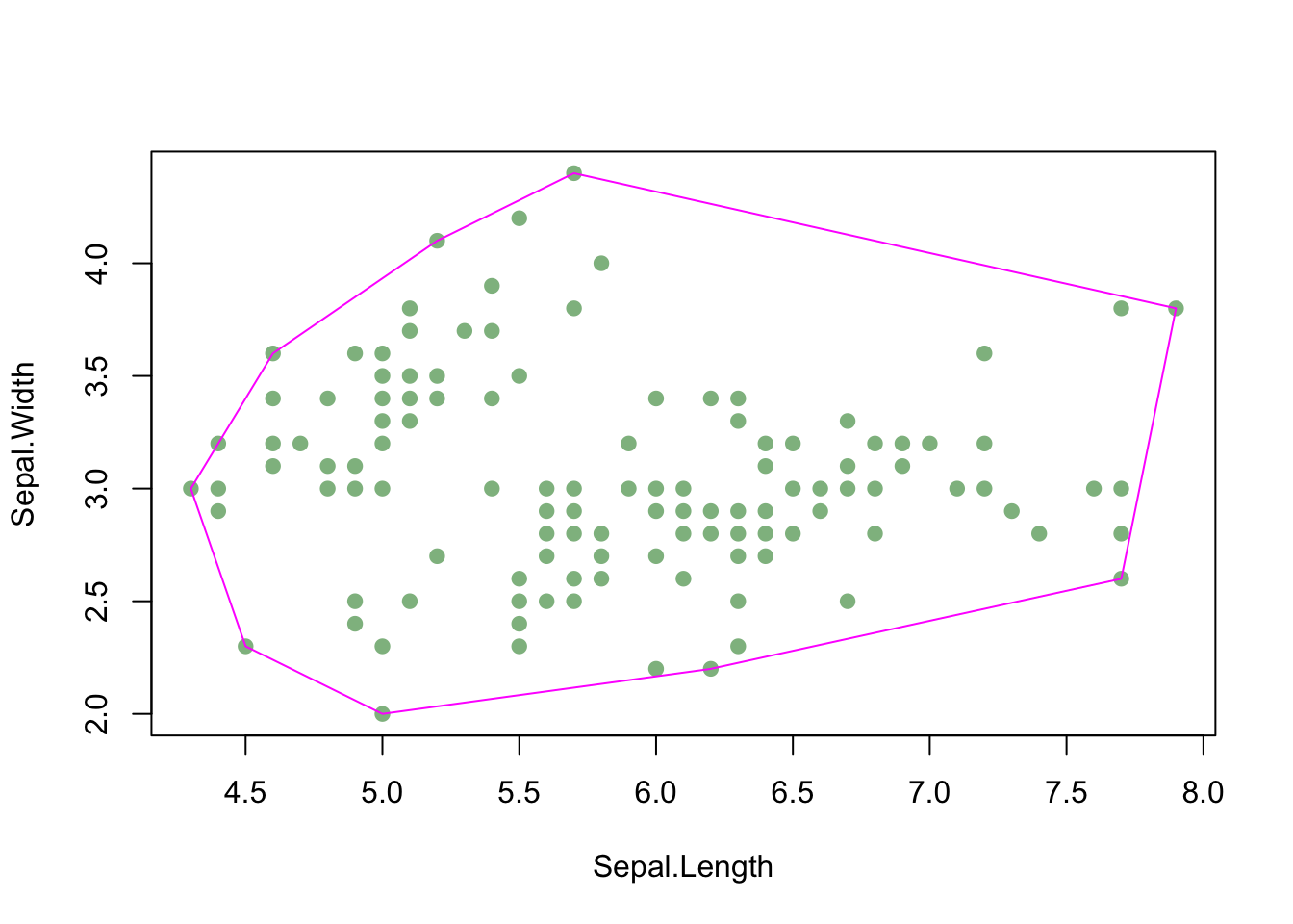
This convex hull (drawn in magenta) is an example of an α-shape: all convex hulls are α-shapes, but not all α-shapes are convex hulls. An α-shape doesn’t have to be convex – the lines making up the border of the shape can create concave edges relative to the points in the dataset. For example:
# create a three-paneled figure
par(mfrow = c(1,3))

# create three different alpha shapes
alphashape_0.5 <- ashape(iris_sepals, alpha = 0.5)
alphashape_1 <- ashape(iris_sepals, alpha = 1)
alphashape_2 <- ashape(iris_sepals, alpha = 2)

# plot alpha = 0.5
plot(iris_sepals, pch = 19, col = "darkseagreen")
plot(alphashape_0.5, col = "magenta", add = TRUE)
# plot alpha = 1
plot(iris_sepals, pch = 19, col = "darkseagreen")
plot(alphashape_1, col = "magenta", add = TRUE)
# plot alpha = 2
plot(iris_sepals, pch = 19, col = "darkseagreen")
plot(alphashape_2, col = "magenta", add = TRUE)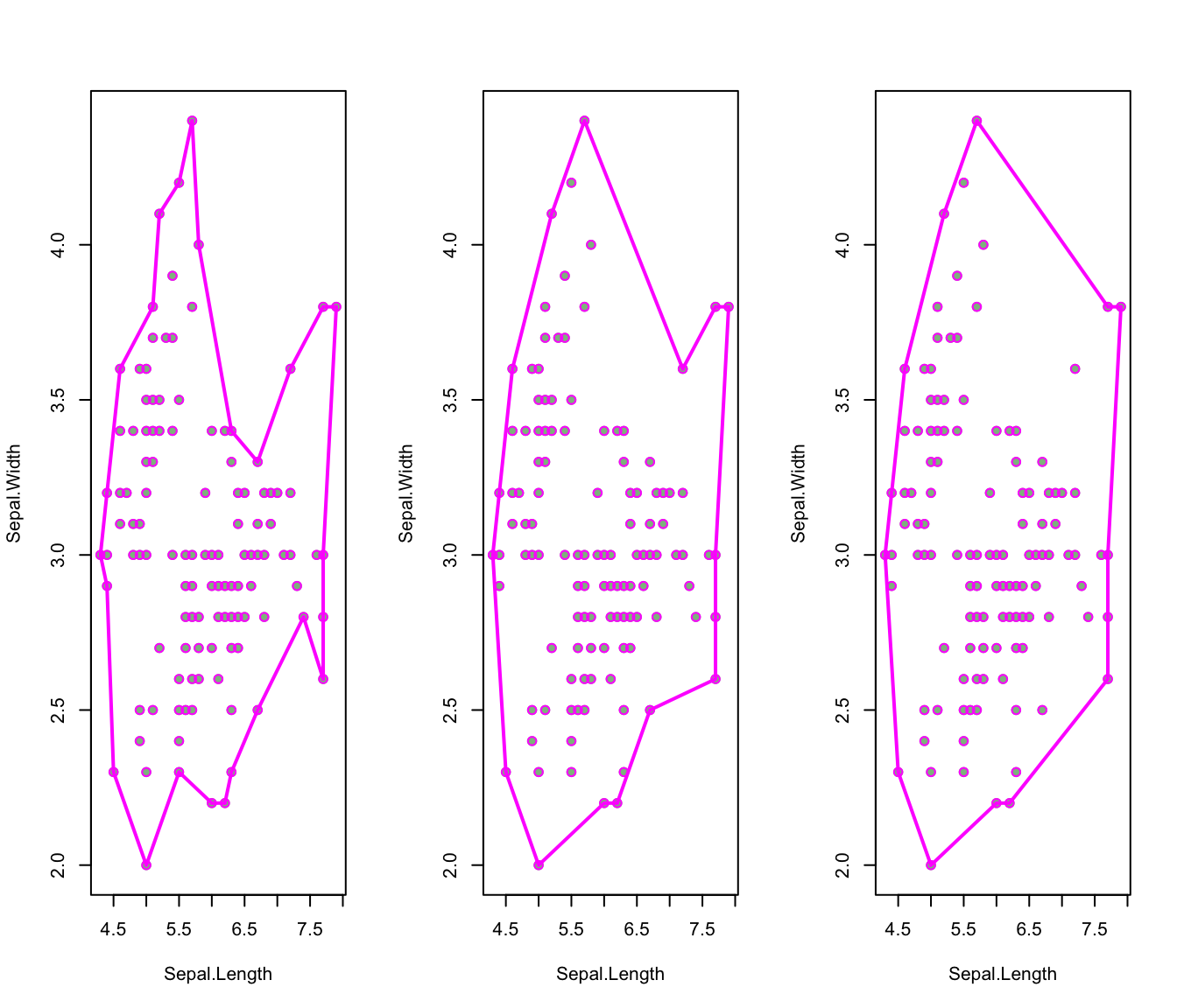
# reset plotting parameters
par(mfrow = c(1,1))
Alpha shapes are created using the ashape function from the alphahull package. As you can see, increasing the α value makes the shape closer and closer to the convex hull, while low values of α make the shape more concave.
Alpha shapes to polygons
In order to use α-shapes with spatial data in R, I wanted to convert these shapes to polygons. To accomplish this, I modified some of the code from an RPubs by Barry Rowlingson to create the following function:
library(igraph)
## Warning: package 'igraph' was built under R version 3.5.2
##
## Attaching package: 'igraph'
## The following objects are masked from 'package:stats':
##
##     decompose, spectrum
## The following object is masked from 'package:base':
##
##     union

ashape2poly <- function(ashape){
  # Convert node numbers into characters
  ashape$edges[,1] <- as.character(ashape$edges[,1])
  ashape_graph <- graph_from_edgelist(ashape$edges[,1:2], directed = FALSE)
  if (!is.connected(ashape_graph)) {
    stop("Graph not connected")
  }
  if (any(degree(ashape_graph) != 2)) {
    stop("Graph not circular")
  }
  if (clusters(ashape_graph)$no > 1) {
    stop("Graph composed of more than one circle")
  }
  # Delete one edge to create a chain
  cut_graph <- ashape_graph - E(ashape_graph)[1]
  # Find chain end points
  ends = names(which(degree(cut_graph) == 1))
  path = get.shortest.paths(cut_graph, ends[1], ends[2])$vpath[[1]]
  # this is an index into the points
  pathX = as.numeric(V(ashape_graph)[path]$name)
  # join the ends
  pathX = c(pathX, pathX[1])
  return(pathX)
}
For the reasoning behind the function, check out the RPubs I referred to for guidance. For a sanity check, we can compare the resulting shape to the original α-shape we were trying to replicate:
alphapoly_1 <- ashape2poly(alphashape_1)
plot(iris_sepals, pch = 19, col = "darkseagreen")
# show the original alpha shape
plot(alphashape_1, lwd = 5, col = "gray", add = TRUE)
# plot the new polygon
lines(iris_sepals[alphapoly_1, ], col = "magenta")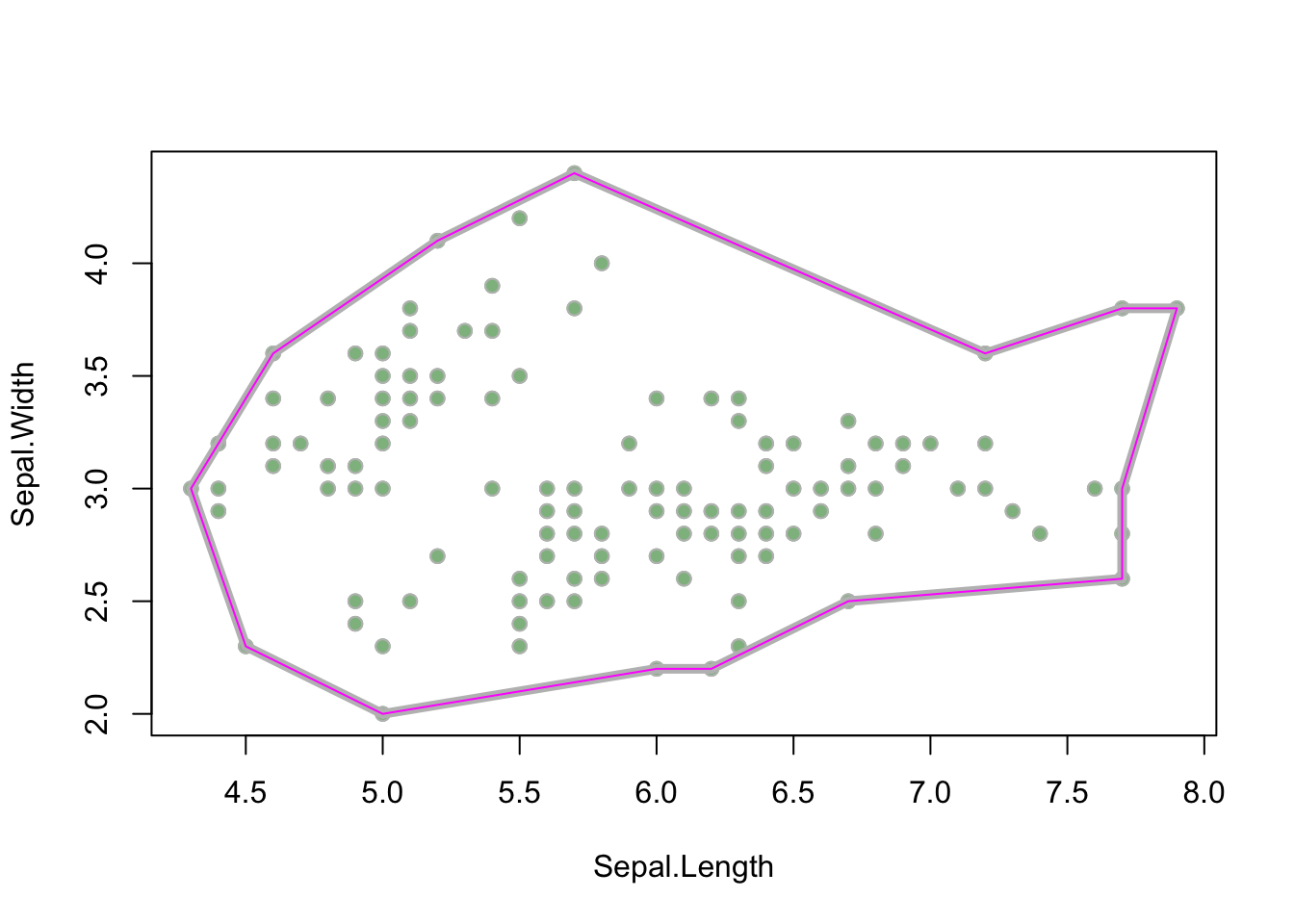
Alpha hulls
Alpha hulls add another layer of complexity to this process because they can include curved lines (arcs) as edges of a shape. For example:
alphahull_1 <- ahull(iris_sepals, alpha = 1)

plot(iris_sepals, pch = 19, col = "darkseagreen")
plot(alphahull_1, col = "magenta", add = TRUE)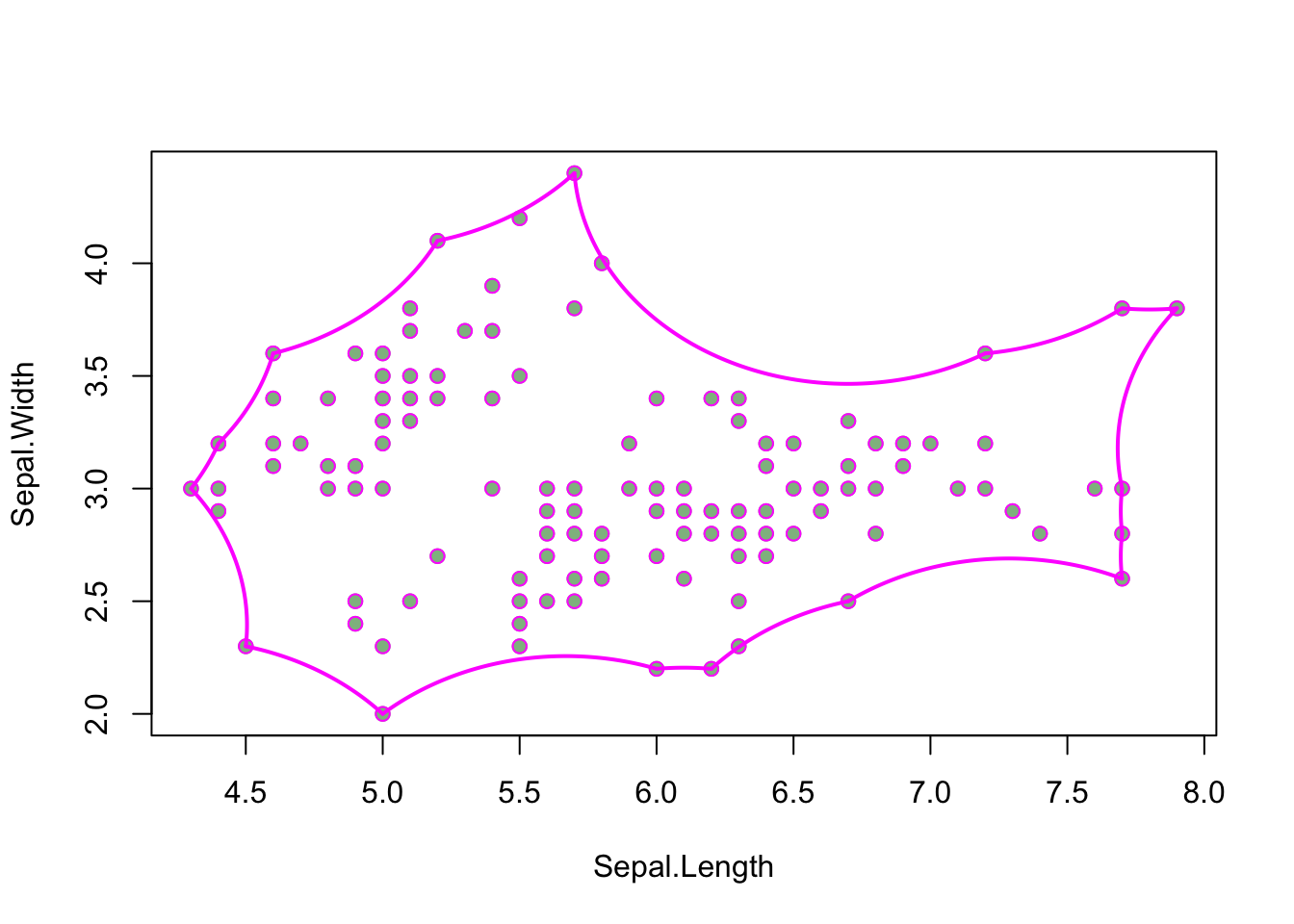
Arcs to lines
To deal with this curvature, I wrote the following function to convert the arcs between points in the hull to a series of very short line segments in order to approximate the curve.
# function to convert an arc into line segments
# given the center of the arc, the radius, the vector, and the angle (radians)
arc2line <- function(center, r, vector, theta, npoints = 100) {
  # Get the angles at the extremes of the arcs
  angles <- anglesArc(vector, theta)
  # Generate sequence of angles along the arc to determine the points
  seqang <- seq(angles[1], angles[2], length = npoints)
  # Generate x coordinates for points along the arc
  x <- center[1] + r * cos(seqang)
  # Generate y coordinates for points along the arc
  y <- center[2] + r * sin(seqang)
  coords.xy <- cbind(x,y)
  line <- Line(coords = coords.xy)
  return(line)
}
Hulls to lines
Using the previous function, I wrote another function to take an α-hull and convert it into a set of SpatialLines objects. The function uses the arc2line function from above to convert each arc in the α-hull into a series of lines, before adding each of these sets of lines together. (This function was updated on 6 January 2021 based on my response to kostas_k84 – thank you to everyone who brought this up to me!)
ahull2lines <- function(hull){
  arclist <- hull$arcs
  lines <- list()
  for (i in 1:nrow(arclist)) {
    # Extract the attributes of arc i
    center_i <- arclist[i, 1:2]
    radius_i <- arclist[i, 3]
    vector_i <- arclist[i, 4:5]
    theta_i <- arclist[i, 6]
    # Convert arc i into a Line object
    line_i <- arc2line(center = center_i, r = radius_i, vector = vector_i, theta = theta_i)
    list_length <- length(lines)
    if(list_length > 0){
      # If a line has already been added to the list of lines
      # Define last_line_coords as the coordinates of the last line added to the list before the ith line
      last_line_coords <- lines[[list_length]]@coords
    }
    if(i == 1){
      # Add the first line to the list of lines
      lines[[i]] <- line_i
    } else if(isTRUE(all.equal(line_i@coords[1,], last_line_coords[nrow(last_line_coords),]))){
      # If the first coordinate in the ith line is equal to the last coordinate in the previous line
      # then those lines should be connected
      # Row bind the coordinates for the ith line to the coordinates of the previous line in the list
      lines[[list_length]]@coords <- rbind(last_line_coords, line_i@coords[2:nrow(line_i@coords),])
    } else {
      # If the first coordinate in the ith line does not match the last coordinate in the previous line
      # then the ith line represents a new line
      # Add the ith line to the list as a new element
      lines[[length(lines) + 1]] <- line_i
    }
  }
  # Convert the list of lines to a Line object
  lines <- Lines(lines, ID = 'l')
  # Convert the Line object to a SpatialLines object
  sp_lines <- SpatialLines(list(lines))
  return(sp_lines)
}
The results look like this:
lines_1 <- ahull2lines(alphahull_1)
# the result is a SpatialLines object
class(lines_1)
## [1] "SpatialLines"
## attr(,"package")
## [1] "sp"

plot(iris_sepals, pch = 19, col = "darkseagreen")
# show the original alpha shape
plot(alphahull_1, lwd = 5, col = "gray", add = TRUE)
# plot the new polygon
plot(lines_1, col = "magenta", add = TRUE)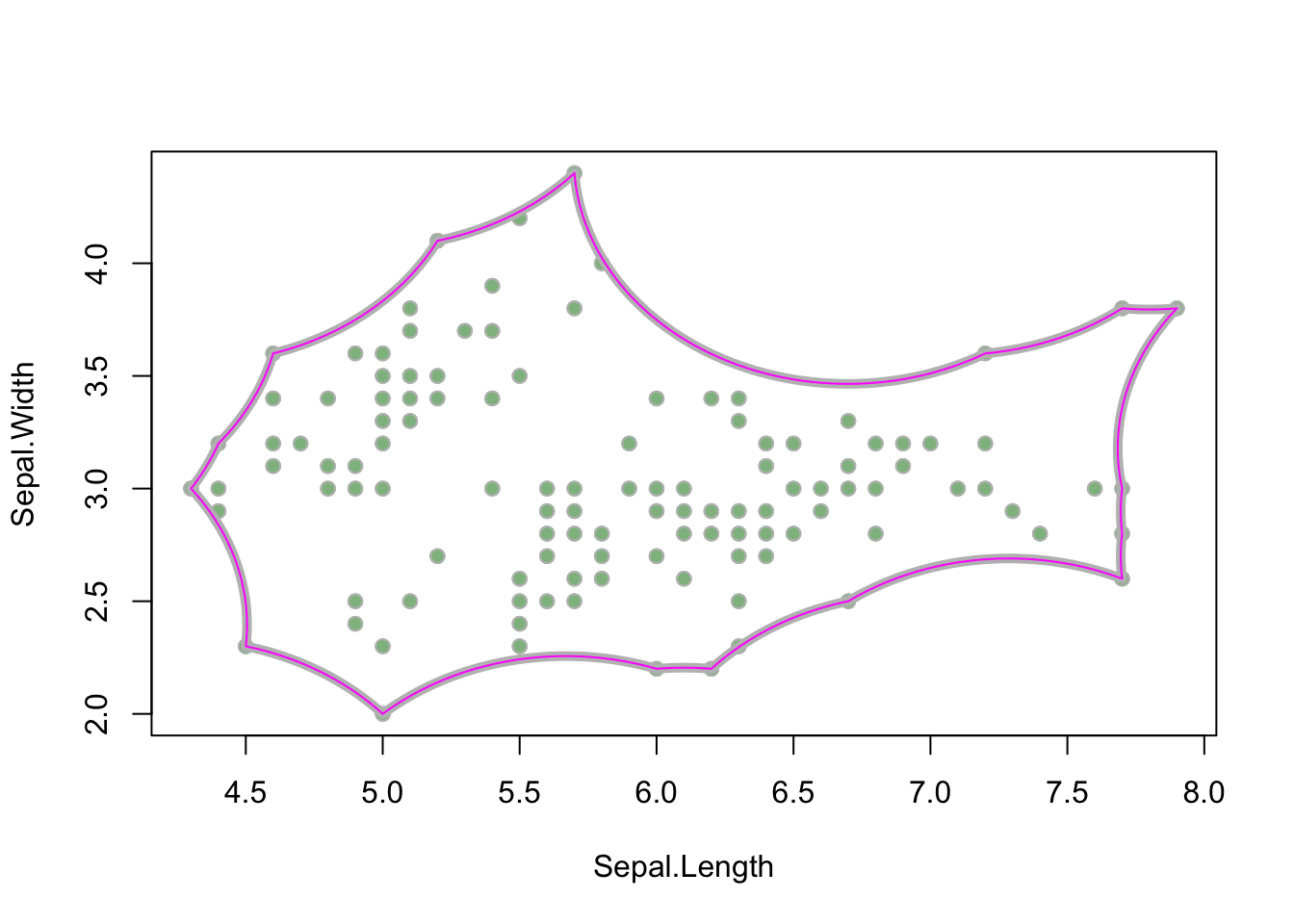
The resulting SpatialLines object is an almost spot-on approximation of the original α-hull (shown in gray).
SpatialLines to SpatialPolygon
Now, I needed a way to convert the SpatialLines object into a SpatialPolygon that would cover the same shape as the original α-hull. To accomplish this, I wrote a function that takes a SpatialLines object, checks which lines are part of polygons (i.e. form closed shapes), and converts those polygons to a SpatialPolygon.
spLines2poly <- function(sp_lines){
  # Extract the lines slot
  lines_slot <- sp_lines@lines[[1]]
  # Create a list of booleans indicating whether a given Line represents a polygon
  poly_bool <- sapply(lines_slot@Lines, function(x){
    coords <- lines_slot@Lines[[1]]@coords
    # Check if the first coordinate in the line is the same as the last
    all.equal(coords[1,], coords[nrow(coords),])
  })
  # Pull out the lines that form polygons
  poly_lines <- sp_lines[poly_bool]
  poly_lines_slot <- poly_lines@lines
  # Create SpatialPolygons
  sp_polys <- SpatialPolygons(list(Polygons(lapply(poly_lines_slot, function(x) {
    Polygon(slot(slot(x, "Lines")[[1]], "coords"))
  }), ID = "1")))
  return(sp_polys)
}
We can apply this function to the lines_1 object we made from the original alphahull_1:
SpPoly_1 <- spLines2poly(lines_1)
class(SpPoly_1)
## [1] "SpatialPolygons"
## attr(,"package")
## [1] "sp"

plot(iris_sepals, pch = 19, col = "darkseagreen")
# show the original alpha shape
plot(alphahull_1, lwd = 5, col = "gray", add = TRUE)
# plot the new polygon
plot(SpPoly_1, border = "magenta", add = TRUE)
Alpha hulls to SpatialPolygons
Finally, we can string all of those functions together to create a single function that will convert an α-hull directly into a SpatialPolygon:
ahull2poly <- function(hull){
  # Convert the alpha hull to SpatialLines
  hull2SpatialLines <- ahull2lines(hull)
  # Convert SpatialLines to SpatialPolygon
  SpatialLines2SpatialPolygon <- spLines2poly(hull2SpatialLines)
  return(SpatialLines2SpatialPolygon)
}
As a final sanity check, we can see that the resulting shape is the same as the original shape produced by the alphahull package:
hullpoly_1 <- ahull2poly(alphahull_1)
class(hullpoly_1)
## [1] "SpatialPolygons"
## attr(,"package")
## [1] "sp"

plot(iris_sepals, pch = 19, col = "darkseagreen")
# show the original alpha shape
plot(alphahull_1, lwd = 5, col = "gray", add = TRUE)
# plot the new polygon
plot(hullpoly_1, border = "magenta", add = TRUE)
GitHub
The code for these functions is on my GitHub at https://github.com/babichmorrowc/hull2spatial. If you have any thoughts or suggestions, please comment on this post or submit a pull request on GitHub. I hope to be formulating these functions into a package in the near future, so stay tuned!
Citations
Beatriz Pateiro-Lopez and Alberto Rodriguez-Casal. (2016). alphahull: Generalization of the Convex Hull of a Sample of Points in the Plane. R package version 2.1. https://CRAN.R-project.org/package=alphahull
- Posted on:
- March 18, 2019
- Length:
- 9 minute read, 1902 words
- Categories:
- R species distribution modeling