brat and it's the same but it's a blog post so it's not
How brat is this color?
By Cecina Babich Morrow in R
August 17, 2024
Inspiration for this post

In this case, my muse for this post is probably pretty clear. I am doing my best to have a brat summer, as are we all. But of course, the question that comes to mind is…how brat is my summer, really?
While most aspects of brat are unquantifiable, that iconic green seemed like a potential place to start. I had the idea of entering the hex code for a color and spitting out a number telling you how close your color was to brat color. The journey turned out to be a bit more complicated than that.
What color is brat?
Of course the first question was what color brat is, exactly. I used Digital Colour Meter to determine the color on the essential https://www.bratgenerator.com/ (making sure it was in green mode, since black and white just isn’t as interesting).
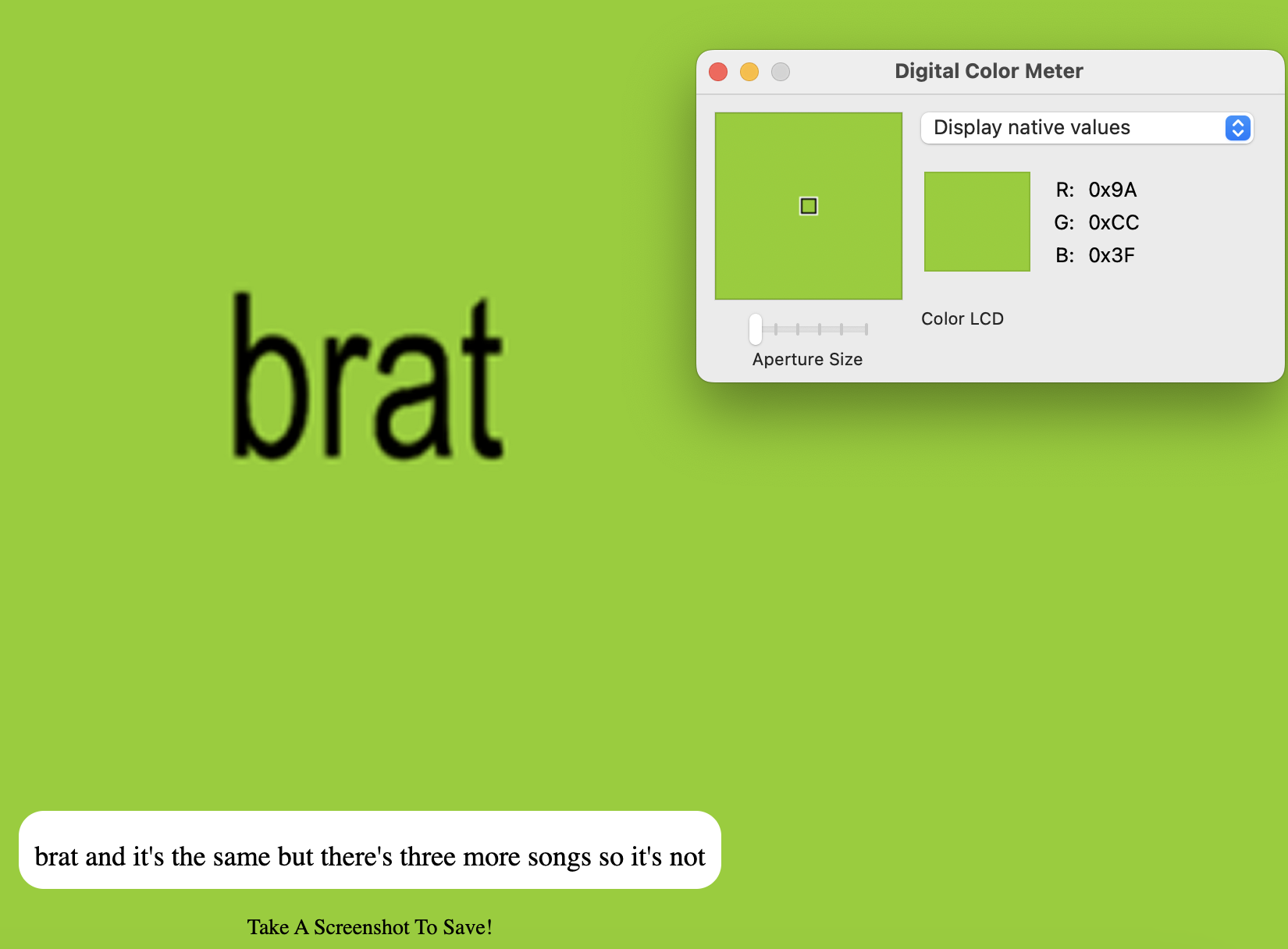
Based on this investigative reporting, I came up with the hex code #9ACC3F. However, I’m nothing if not thorough, so I wanted to check my work. I did the same to the album cover color on Spotify, this time coming up with #99CB3F. Aggravating.
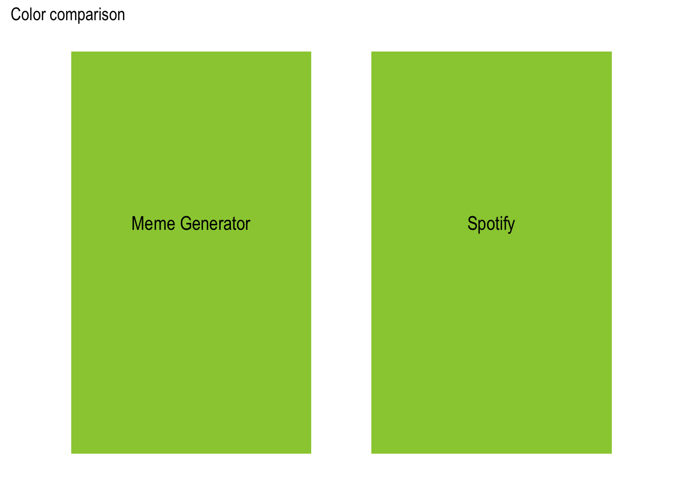
At the end of the day, my untrained eye can’t really distinguish these two, even after the brain-rotting number of hours I’ve spent staring at this album. I’m going with the meme generator hex code for this.
Color distance
I assumed I could do a quick distance calculation in color space to determine the distance of any color to brat color.
RGB
RGB space seemed like the ideal way to do this. The RGB color model essentially adds together the red, green, and blue components by superimposing to create a color or image. Each of the three colors can be anywhere between fully on and fully off. When they’re all fully on, we get white; all fully off gives black.
This seemed like a fabulous way to generate a space on which to measure color distance. I could simply define a cube with three axes representing red, green, and blue, and then calculate the Euclidean distance between points in that space.
For more delightful RGB fun facts, there is a trusty Wikipedia article where you can learn about everything from the human eye to the first permanent color photograph.
Let’s write an R function that can take two colors and calculate the distance between them in this RGB “cube”. We’ll assume we want to do everything in hex codes (we can extend this later if we want). I like the idea of returning the percentage of brat-ness, so we’ll convert the Euclidean distance into the percentage of the maximum distance in a unit cube ($\sqrt 3$).
color_distance <- function(ref_color = "#9ACC3F",
                           new_color,
                           color_space = "rgb") {
  # Convert hex to rgb
  # Using row vectors to work well with dist in the next step
  # Dividing by 255 to get a unit cube
  ref_rgb <- t(col2rgb(ref_color)) / 255
  new_rgb <- t(col2rgb(new_color)) / 255

  # Calculate euclidean distance between colors
  dist <- as.numeric(dist(rbind(new_rgb, ref_rgb)))

  # Calculate percent of sqrt 2
  perc_dist <- 1 - dist / sqrt(3)
  return(perc_dist)
}
Let’s test it out:
brat_hex <- "#9ACC3F"
bi_hex <- "#D60270"
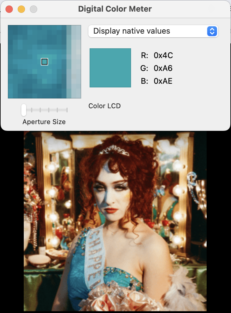
midwest_hex <- "#4CA6AE"
# How brat is the brat color?
brat_dist <- color_distance(new_color = brat_hex)
# How brat is #D60270?
bi_dist <- color_distance(new_color = bi_hex)
# How brat is #4CA6AE?
midwestprincess_dist <- color_distance(new_color = midwest_hex)
So according to Euclidean distance in the unit RGB cube, the brat color is 100% brat, this color lifted from the bisexual pride flag is 51.02% brat, and this color lifted from The Rise and Fall of a Midwest Princess album cover is 68.1% brat.
We can visualize the relative positions of the colors in our cube like so:
HSV
What if we aren’t feeling particularly cubic? An alternative to the RGB cube representation is instead depicting colors located in a cylinder. This can be done in a couple different ways: HSL (hue, saturation, lightness), HSV (hue, saturation, value), or HSI (hue, saturation, intensity). This Wikipedia page has a great explanation of each, so I won’t go into the distinctions too much. Instead, I’ve decided to go with HSV purely because I think the cylinder looks coolest (please debate me on this).
HSV situates the hue of a color around the circular dimension of the cylinder, radiating from red to green to blue back to red. As you move from the center of the cylinder outwards, the colors become more saturated, and as you move from the bottom of the cylinder upwards, the colors become lighter.
As a (non-)expert, I think a crucial part of the brat color appeal is the level of saturation, so I was interested in seeing if a color schema that explicitly accounts for saturation would give some different brat levels. Let’s expand our function:
hsv2cyl_xyz <- function(hsv_vec) {
  # Given a 3x1 matrix, e.g. one returned by rgb2hsv
  # Assuming the 1st value is hue, 2nd saturation, 3rd value
  xyz_coord <- c(hsv_vec[2] * cos(hsv_vec[1] * 2 * pi),
                 hsv_vec[2] * sin(hsv_vec[1] * 2 * pi),
                 hsv_vec[3])
  return(xyz_coord)
}

color_distance <- function(ref_color = "#9ACC3F",
                           new_color,
                           color_space = "rgb") {

  # Convert hex to rgb
  # Dividing by 255 to get a unit cube
  ref_rgb <- col2rgb(ref_color) / 255
  new_rgb <- col2rgb(new_color) / 255

  if(color_space == "rgb") {
    # Calculate euclidean distance between colors
    dist <- as.numeric(dist(rbind(t(new_rgb), t(ref_rgb))))

    # Calculate percent of sqrt 3
    perc_dist <- 1 - dist / sqrt(3)
  } else if(color_space == "hsv") {
    # Convert hex to hsv
    ref_hsv <- rgb2hsv(ref_rgb, maxColorValue = 1)
    new_hsv <- rgb2hsv(new_rgb, maxColorValue = 1)

    # Convert HSV to xyz coordinates in the cylinder
    ref_xyz <- hsv2cyl_xyz(ref_hsv)
    new_xyz <- hsv2cyl_xyz(new_hsv)

    # Calculate euclidean distance between colors
    dist <- as.numeric(dist(rbind(ref_xyz, new_xyz)))

    # Calculate percent of sqrt 5
    perc_dist <- 1 - dist / sqrt(5)
  }

  return(perc_dist)
}
So let’s calculate the brat percentages using HSV instead:
# How brat is the brat color?
brat_dist_hsv <- color_distance(new_color = brat_hex, color_space = "hsv")
# How brat is #D60270?
bi_dist_hsv <- color_distance(new_color = bi_hex, color_space = "hsv")
# How brat is #4CA6AE?
midwestprincess_dist_hsv <- color_distance(new_color = midwest_hex, color_space = "hsv")
In our HSV cylinder, the brat color is 100% brat, the bi flag color is 37.03% brat (13.99 percentage points lower than in RGB space), and the Midwest Princess color is 55.45% brat (12.65 percentage points lower).
Let’s see the relative positions on our cylinder:
Perceptual uniformity
As fun as the cube and cylinder were to create, both RGB and HSV have a big downside: they lack ✨ perceptual uniformity ✨. What this means is that moving an equal Euclidean distance in the RGB cube or the HSV cylinder doesn’t translate to a linear change in the hue according to the human eye. This article has some great visualizations of the problem. Since we’re trying to measure distance from brat according to the human eye, we need a new approach.
Apparently fixing this issue is an actual nightmare, spawning a dizzying array of different color spaces and distance metrics. Some (but probably not all) of these are outlined in the Wikipedia color distance article. I’ll do my best to talk through one such solution here.
CIELAB
The International Commission on Illumination (CIE) developed a new color space called CIELAB. CIELAB uses three values: perceptual lightness \(L^*\), as well as \(a^*\) and \(b^*\) for the red - green and blue - yellow axes.
CIE’s mission statement is “Advancing knowledge and providing standardization to improve the lighted environment”. I for one am comforted that people are dedicated to this.
We can see this funky-looking space here:
Spoiler alert, CIELAB is still not perceptually uniform. Best of luck to CIE in their ongoing quest in what is apparently a very difficult quest. For the purposes of brat, we soldier on with what has already been created.
\(\Delta E^*\)
In addition to CIELAB, CIE also created a distance metric called \(\Delta E^*\), which attempts to measure the difference between colors according to human perception. The formula has been tweaked several times, yielding a 1976 version, a 1984 version, a 1994 version, and a 2000 version. We’ll go with the most recent. I won’t go through the math, but suffice it to say there are at least 11 lines of equations (see this
Delta E 101 article). Fortunately, the
farver R package has done the delightful work of coding up these equations, so we can go ahead and just borrow their compare_colour function here.
\(\Delta E^*\) values range from 0 to 100, with the following interpretations (from
this post):
| Delta E | Perception |
|---|---|
| <= 1.0 | Not perceptible by human eyes. |
| 1 - 2 | Perceptible through close observation. |
| 2 - 10 | Perceptible at a glance. |
| 11 - 49 | Colors are more similar than opposite. |
| 100 | Colors are exact opposite. |
We’ll find the \(\Delta E^*\) between our three colors and the original brat color (then we can find the brat percentage by subtracting from 100):
library(farver)
# How brat is the brat color?
brat_dist_de <- compare_colour(from = t(brat_rgb) * 255,
                               to = t(brat_rgb) * 255,
                               from_space = "rgb",
                               method = "cie2000")
# How brat is #D60270?
bi_dist_de <- compare_colour(from = t(brat_rgb) * 255,
                               to = t(bi_rgb) * 255,
                               from_space = "rgb",
                               method = "cie2000")
# How brat is #4CA6AE?
midwestprincess_dist_de <- compare_colour(from = t(brat_rgb) * 255,
                               to = t(midwest_rgb) * 255,
                               from_space = "rgb",
                               method = "cie2000")
Using \(\Delta E^*\), the brat color is 100% brat, this color lifted from the bisexual pride flag is 19.77% brat, and this color lifted from The Rise and Fall of a Midwest Princess album cover is 63.87% brat. We find that the bi pride color is more opposite brat than similar, while the Midwest Princess color is more similar than opposite.
We can visualize the relative positions of these colors in CIELAB space now:
What have we accomplished?
To be honest, it’s unclear. I have had a wonderful time, and in the end, is that not what brat summer is all about?
At the very least, we now have the ability to determine relative brat-ness of different colors in a variety of spaces:
Beyond this vital information, I have delved into a tiny fraction of the insanely complex world of color, while listening to the album of the summer an unconscionable number of times, so I’m counting this as a win.
What’s next?
Now that I have descended down this colorful rabbithole, my dream is to make a Shiny app that can tell you how brat a color is given its hex code, with the option of a variety of color spaces/distance metrics. Then, in the ultimate dream, I wish to be able to take an image and tell you how brat the entire photo is based on color (the brat-ness of the image content seems like your business to determine). These both seem like worthy endeavors in the sport of Productive Procrastination, so stay tuned. My father informed me this morning that brat summer is over, so I may have missed the boat on these, but I have been adamantly asserting since July that this album is Not a Phase But Rather Who I am Now, so might as well put my coding skills where my mouth is. If you are interested in this, fantastic. If not, in the words of Charli,
Resources
- The all-important brat generator
- Wikipedia’s RGB color model article
- Wikipedia’s HSL and HSV article
- Wikipedia’s Color distance article
- Programming Design System’s Perceptually uniform color spaces
- Steve Hanov’s article Fun with Colour Difference
- Zachary Schuessler’s article Delta E 101