Least squares regression: Part 2

Inspiration for this post

Following up on my last post about least-squares regression, here’s part 2, where we cover feature transformation, the dangers of over-fitting, and a possible solution in the form of cross-validation. As before, most of the material I’m showing comes from a class I took with Dr. Song Liu.

Feature transformation

Since we are often living in a non-linear world, linear least-squares might not cut it. To address this issue, we can apply a feature transform to the input variables before we apply least squares. We define a new prediction function \(f'(\textbf{x};\textbf{w}) := \langle\textbf{w}_1, \phi(\textbf{x})\rangle + w_0\) using a feature transform \(\phi(\textbf{x}): \mathbb{R}^d \rightarrow \mathbb{R}^b\) with degree \(b\). Then minimizing the sum of squared errors yields \(\textbf{w}_{LS}=(\phi(\textbf{X})\phi(\textbf{X})^\top)^{-1}\phi(\textbf{X})\textbf{y}^\top\). If \(\phi(\textbf{X})\) is symmetric and invertible, then we can simplify further:

::: {.theorem name=“Least squares with a feature transform”} If \(\phi(\textbf{X})\) is symmetric and invertible, then \(\textbf{w}_{LS}=[\phi(\textbf{X})]^{-1}\textbf{y}^\top\) :::

::: {proof} \begin{align*} \textbf{w}\_{LS} &= \[\phi(\textbf{X})\phi(\textbf{X})^\top\]^{-1}\phi(\textbf{X})\textbf{y}^\top \\ &= \[\phi(\textbf{X})^\top\]^{-1}\[\phi(\textbf{X})\]^{-1}\phi(\textbf{X})\textbf{y}^\top \\ &= \[\phi(\textbf{X})^\top\]^{-1}\textbf{y}^\top \\ &= \[\phi(\textbf{X})\]^{-1}\textbf{y}^\top \end{align*}

■ :::

R implementation

In the last post, we created two functions: least_squares_solver() to find \(\textbf{w}_{LS}\) and least_squares_predict() to make predictions using the coefficients we calculate on a new dataset. We’re going to need to extend these functions to handle the extensions we’re making. First, we’ll allow our functions to accommodate polynomial feature transformation of the form \(\phi(\textbf{x}) = [\textbf{x}, \textbf{x}^2, \textbf{x}^3, ..., \textbf{x}^b]^\top\):

least_squares_solver_ft <- function(input_variables,
                                    output_variable, 
                                    b = 1) {
  # Set up variables
  y <- output_variable
  phi_X <- t(as.matrix(input_variables^b)) # convert each x_i into column vector
  power <- b - 1
  while(power > 0) {
    phi_X <- rbind(phi_X, t(as.matrix(input_variables^power)))
    power <- power - 1
  }
  # Add intercept
  phi_X <- rbind(phi_X, rep(1, ncol(phi_X)))
  
  # Compute w_LS
  w_LS <- solve(phi_X %*% t(phi_X)) %*% phi_X %*% as.matrix(y)
  return(w_LS)
}

# Function to apply coefficients to a new set of data
least_squares_predict_ft <- function(input_variables,
                                     coefficients,
                                     b = 1) {
  # Set up variables
  phi_X <- t(as.matrix(input_variables^b)) # convert each x_i into column vector
  power <- b - 1
  while(power > 0) {
    phi_X <- rbind(phi_X, t(as.matrix(input_variables^power)))
    power <- power - 1
  }
  # Add intercept
  phi_X <- rbind(phi_X, rep(1, ncol(phi_X)))
  
  preds <- t(as.matrix(coefficients)) %*% phi_X
  return(preds)
}

# Function to calculate sum of squared errors
sum_squared_errors <- function(prediction, actual) {
  squared_error <- (actual - prediction)^2
  return(sum(squared_error))
}

Overfitting

By introducing more complex feature transformations, we encounter the trade-off between model flexibility and the generalizability of our predictions. As the degree \(b\) of our feature transformation function \(\phi(\textbf{X})\) increases, our prediction function becomes more and more flexible. we can quantify this problem, known as overfitting, by computing \(\textbf{w}_{LS}\) on one portion of our data and testing it out on a different part of the data to determine how generalizable our predictions are to unseen data. We split our dataset \(D\) at random into a training dataset \(D_0\) and a testing dataset \(D_1\) and fit the model on \(D_0\) alone.

Assumption alert: Note that this process depends on the assumption that our dataset contains IID pairs of input and output variables. This assumption does not hold for series data, for instance.

This process allows us to calculate two measurements of how well our model is doing: (1) training error, how well our model predicts the data \(D_0\) on which it was trained, and (2) testing error, how well the model predicts data on which it was not trained, i.e. generalization. As \(b\) increases, training error continues to decrease as our model becomes increasingly flexible to the data on which it was trained. At first, testing error decreases while \(b\) increases, but past a certain value of \(b\), testing error increases once again as our prediction function loses generalization, meaning that our model is overfitting.

Example

To see this in action, let’s try our new least_squares_solver_ft() function on a randomly generated dataset:

library(ggplot2)

# Generate data ----------------------------------------------------------------
set.seed(42)
# x_i uniformly generated (0,2)
x <- runif(200, min = 0, max = 2)
epsilon <- rnorm(200, mean = 0, sd = 24)
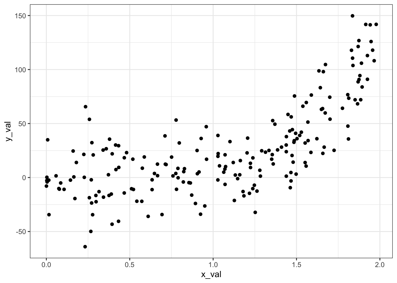
y <- exp(3*x - 1) + epsilon
generated_data <- data.frame(x_val = x, y_val = y)

# Visualize
ggplot(data = generated_data, aes(x = x_val, y = y_val)) +
  geom_point() +
  theme_bw()

We’ll start with running a standard linear least squares, equivalent to a feature transform where \(b = 1\):

# Model with b = 1 -----------------------------------------------------
# Fit linear least squares on the training data
least_squares_1 <- least_squares_solver_ft(generated_data$x_val,
                                           generated_data$y_val,
                                           b = 1)

# Apply the model to the testing data
preds_1 <- least_squares_predict_ft(generated_data$x_val, least_squares_1)
generated_data$preds_1 <- as.vector(preds_1)
# Calculate error
error_1 <- sum_squared_errors(preds_1, generated_data$y_val)
error_1

## [1] 179048.1

We can visualize our results:

library(ggplot2)

ggplot(data = generated_data) +
  geom_point(aes(x = x_val, y = y_val)) +
  geom_line(aes(x = x_val, y = preds_1), color = "red") +
  theme_bw()

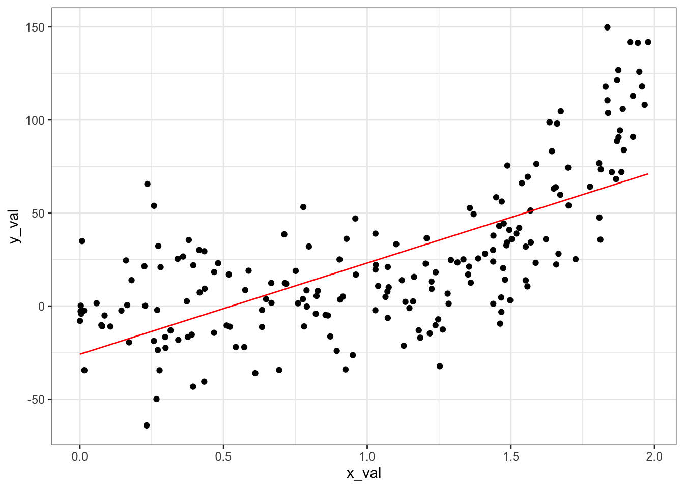
We’re clearly not capturing the non-linear pattern in the data very well. Let’s try a very flexible feature transformation with \(b = 9\) to see if that addresses our problem:

# Model with b = 9 -----------------------------------------------------
# Fit linear least squares on the training data
least_squares_9 <- least_squares_solver_ft(generated_data$x_val,
                                           generated_data$y_val,
                                           b = 9)

# Apply the model to the testing data
preds_9 <- least_squares_predict_ft(generated_data$x_val,
                                    least_squares_9,
                                    b = 9)
generated_data$preds_9 <- as.vector(preds_9)
# Calculate error
error_9 <- sum_squared_errors(preds_9, generated_data$y_val)
error_9

## [1] 103317.3

We have a much lower sum of squared errors.

ggplot(data = generated_data) +
  geom_point(aes(x = x_val, y = y_val)) +
  geom_line(aes(x = x_val, y = preds_9), color = "red") +
  theme_bw()

We are seeing some wiggliness (a highly technical term) to our prediction line that we know doesn’t reflect the underlying pattern in our data, however. This indicates overfitting, where our model is too tuned into the random variation in our sample and loses the ability to generalize to unseen data.

Benign overfitting

Typically, we observe this pattern of increasing the complexity of the prediction function first yielding improvements in testing error, and then deteriorated performance as complexity increases past a certain point. This pattern is known as the bias-variance trade-off. As with most things, though, there can be exceptions to this general process.

Typically, we observe this pattern of increasing the complexity of the prediction function first yielding improvements in testing error, and then deteriorated performance as complexity increases past a certain point. This pattern is known as the bias-variance trade-off.

Bartlett et al. (2020) focused on the statistical problem of linear regression to determine whether benign overfitting can occur here as well, and if so, under what conditions. They examine the case where the data has infinite dimension and the prediction function fits the training data exactly. The latter occurs when there are more parameters than datapoints, which can yield multiple solutions which all minimize squared error, so they select the parameter with the smallest norm out of those which yield a training error of zero, a technique known as minimum norm estimation. The authors then characterize situations where the resulting prediction function will have low testing error as well, i.e. when benign overfitting occurs.

The authors find that in order for benign overfitting to occur, the covariance matrix \(\Sigma\) of the input variables needs to meet certain criteria. They define two notions of effective rank defined in terms of the eigenvalues of \(\Sigma\): \(r\), which splits \(\Sigma\) into large and small eigenvalues, and \(R\), which is the effective rank of the subspace corresponding to the smallest eigenvalues. Using these two types of effective rank, they find that the minimum norm estimator has the highest accuracy when \(\Sigma\) has many non-zero eigenvalues compared to the sample size \(n\), the sum of those eigenvalues is small compared to \(n\), and there are many eigenvalues less than or equal to \(\lambda_{k^*}\), the largest eigenvalue such that \(r_{k^*}(\Sigma) \geq bn\). The eigenvalues of the covariance matrix need to decay sufficiently slowly, while still having a relatively low sum. In practice, this means that benign overfitting requires overparameterization, meaning that there are many low-variance directions in the parameter space, such that the covariance matrix has a heavy tail. When the data has infinite dimension, the decay rate of the eigenvalues must be within a much narrower range of values in order to cause benign overfitting. In a finite dimensional space, however, as long as the dimension of the space is growing faster than the sample size, benign overfitting is likely to occur.

Cross-validation

We need some way to find the balance between flexibility and generalizability in our model. We have several potential options of how to apply the concept of training/testing splits. In the simplest method, we can fit \(f_{LS}(b)\) on \(D_0\), compute testing error on \(D_1\), and select the value of \(b\) that yields the lowest testing error. This approach effectively wastes the data in \(D_1\) for validation, however, and since the testing error is random, the selection of \(b\) may be random. To address these issues, we can use a method called cross-validation to find \(b\). We split \(D\) into \(k+1\) disjoint subsets \(D_0...D_k\) (note that \(k\) can be as large as \(n - 1\), which is known as leave-one-out validation). For \(i\in{0,...,k}\), fit \(f_{LS}^{(i)}(b)\) on all subsets except \(D_i\) for all values of \(b\), and then compute the testing error \(E^{(i)}\) using \(D_i\) as the testing data. Then select the value of \(b\) that minimizes the average testing error \(\frac{\sum_i E^{(i)}}{k+1}\).

Cross-validation is not without its drawbacks, however. Not only does it depend on the IID assumption, but it also becomes very computationally expensive, especially as the dimensionality of the dataset increases. When \(\textbf{x} \in \mathbb{R}^d\), then \(\phi(\textbf{x}) \in \mathbb{R}^{db}\), meaning that \(\textbf{w} \in \mathbb{R}^{db+1}\) without any cross-dimensional polynomials. Adding cross-dimensional polynomials, which are useful when the output value depends on the interaction between multiple inputs, can increase the dimensionality of \(\phi(\textbf{x})\) all the way up to \(\mathbb{R}^{db + {d \choose 2}}\). We can include combinations of terms all the way up to \(d\)-plets: \({d \choose 1} + {d \choose 2} + ... + {d \choose d} = 2^d\). Since the sample size needs to match the output dimension of \(\phi(\textbf{x})\) at a minimum, the sample size has to grow exponentially with the dimension of \(\textbf{x}\), as well as with the degree of the feature transform. Practically, we are typically limited by how much data we can realistically collect, as well as by the computing power needed to analyze it. This issue is known (somewhat dramatically) as the curse of dimensionality.

R implementation

We can use 5-fold cross-validation to find the degree \(b\) that gives us the lowest sum of squared errors on our generated dataset:

# Calculate CV error with different values of b ---------------------------
# Use 5-fold cross-validation
# Randomly shuffle the data
generated_data <-  generated_data[sample(nrow(generated_data)),]
folds <- cut(seq(1,nrow(generated_data)), breaks = 5, labels = FALSE)
# Set up feature space
degrees <- 1:9
# Empty dataframe to store cross-validation error
cross_val_results <- data.frame(b = numeric(), cross_val_error = numeric())
# Loop over all b values
for (b in degrees) {
  cv_error <- c()
  for(i in 1:5) {
    test_data <- generated_data[which(folds == i),]
    train_data <- generated_data[which(folds != i),]
    fit_i <- least_squares_solver_ft(train_data$x_val,
                                     train_data$y_val,
                                     b = b)
    pred_i <- least_squares_predict_ft(test_data$x_val, fit_i, b = b)
    error_i <- sum_squared_errors(pred_i, test_data$y_val)
    cv_error <- c(cv_error, error_i)
  }
  overall_error <- mean(cv_error)
  cross_val_results[b,] <- c(b, overall_error)
}

Let’s see the “sweet spot” where we have the lowest cross-validation error:

ggplot(data = cross_val_results, aes(x = b, y = cross_val_error)) +
  geom_point() +
  scale_x_continuous(breaks = 0:10) +
  labs(x = "b", y = "Cross-validation error") +
  theme_bw()

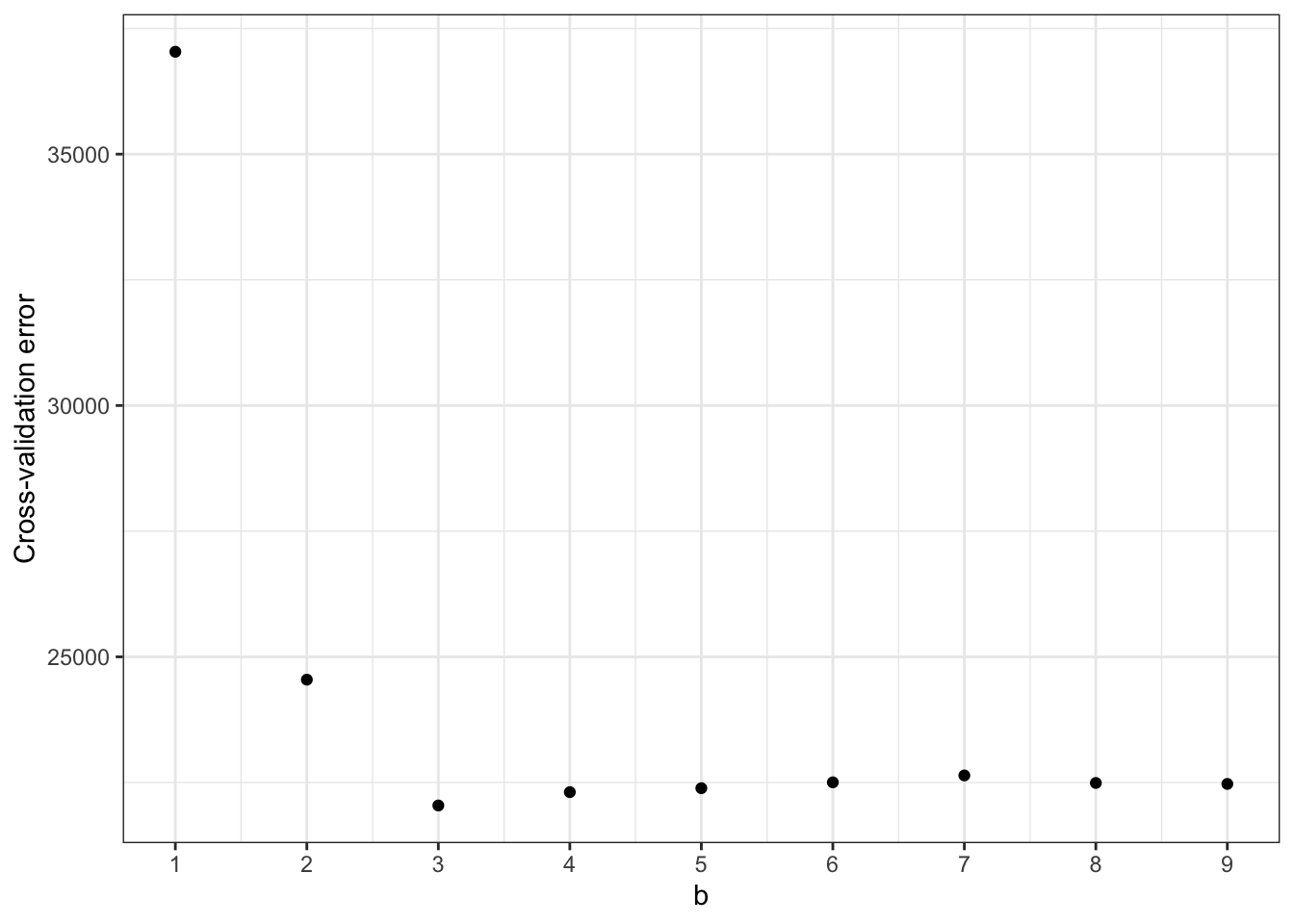
We have the lowest cross-validation error at \(b = 4\). Let’s visualize what that looks like in terms of predictions on our whole dataset:

# Model with b = 4 -----------------------------------------------------
# Fit linear least squares on the training data
least_squares_4 <- least_squares_solver_ft(generated_data$x_val,
                                           generated_data$y_val,
                                           b = 4)

# Apply the model to the testing data
preds_4 <- least_squares_predict_ft(generated_data$x_val,
                                    least_squares_4,
                                    b = 4)
generated_data$preds_4 <- as.vector(preds_4)

# Visualize
ggplot(data = generated_data) +
  geom_point(aes(x = x_val, y = y_val)) +
  geom_line(aes(x = x_val, y = preds_4), color = "red") +
  theme_bw()

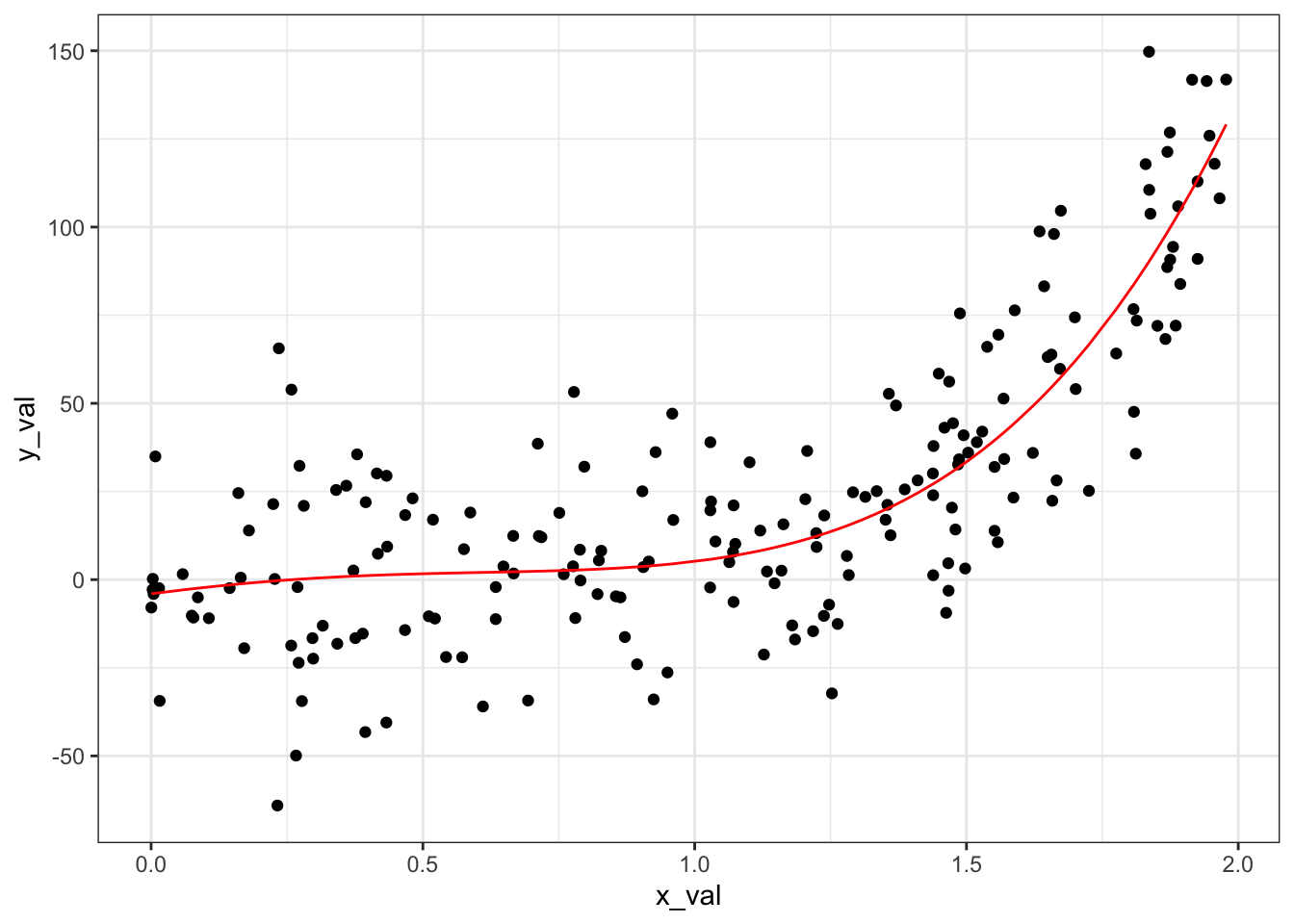
We have successfully de-wiggled our model!

References

Bartlett, P.L., P.M. Long, G. Lugosi, and A. Tsigler. “Benign overfitting in linear regression”, PNAS, 2020.