Hacking Meteorites Part 1: Calculating percent weights

Estimating percent weight of elements in a meteorite.

By Cecina Babich Morrow in hackathon Python

February 20, 2019

Earlier this month I participated in the American Museum of Natural History’s annual hackathon (see my last post for details about the event overall). During the hackathon, I worked with Katy Abbott, another Helen Fellow at the museum with me, to use a machine learning algorithm called DBSCAN to tackle our challenge. This post explains the process we used to complete the first step of the challenge: estimating the percent weights of elements in a meteorite.

Challenge accepted

Our team, consisting of Peter Kang, Jackson Lee, Jeremy Neiman, John Underwood, Katy Abbott, Meret Götschel, and myself, chose to work on the Meteorite Mineral Mapping challenge. For this challenge, our museum stakeholders, Marina Gemma and Sam Alpert, wanted a way to identify the mineral composition of meteorites.

Pixels to percents

The scientists scan meteorites with an electron microprobe, a device that provides the intensity of x-rays emitted from certain elements. The electron microprobe results in images with grayscale intensities corresponding to these x-ray intensities on a pixel-by-pixel basis.

Images of a meteorite produced by the electron microprobe showing pixel intensities for each of 10 elements - brighter grayscale values indicate greater amounts of that element in a pixel.

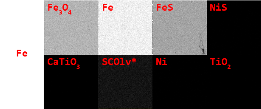
Our first step was to convert these pixel intensities to the percent weight of each element in the mineral at that pixel. To do that, we referred to a set of standard images taken of minerals with a known proportion of each element. For example, the image below shows the pixel intensities of iron in 8 minerals: you can see that the pixels are brightest in Fe, or pure iron, and lower in iron oxide (\(\text{Fe}_3\text{O}_4\)) and troilite, or iron sulfide (FeS).

Standard scan of the intensity of iron in each of 8 known minerals.

We can relate the intensity of the iron pixels in the Fe mineral, for example, to the percent weight in that mineral (100%, since iron is the only element in Fe).

Import data

We started by creating a .csv file with the percent weight of each element in the minderals from the standards:

# import libraries
from sklearn.cluster import DBSCAN as dbscan
from sklearn.linear_model import LinearRegression
import pandas as pd
import numpy as np
from sklearn import metrics
import matplotlib.pyplot as plt
import matplotlib.colors
from sklearn.decomposition import PCA
from pathlib import Path
from skimage.io import imread, imshow
import numpy.ma as ma
from collections import Counter

# read in percent weights by element of the minerals in the standard
weights = pd.read_csv("../../../static/mineralmapping/weights_to_minerals.csv")
print(weights.head())
##        mineral  Mg     Ni  Al        Fe      Ca  Cr   P        S      Ti  Si
## 0  CaTiO3std15 NaN    NaN NaN       NaN  29.481 NaN NaN      NaN  35.211 NaN
## 1  Fe-num2std9 NaN    NaN NaN  100.0000     NaN NaN NaN      NaN     NaN NaN
## 2      FeSstd2 NaN    NaN NaN   63.5252     NaN NaN NaN  36.4748     NaN NaN
## 3   Fe3O4std15 NaN    NaN NaN   72.3591     NaN NaN NaN      NaN     NaN NaN
## 4       Nistd9 NaN  100.0 NaN       NaN     NaN NaN NaN      NaN     NaN NaN

(Note: I was able to add the above Python chunk in R by following these instructions).

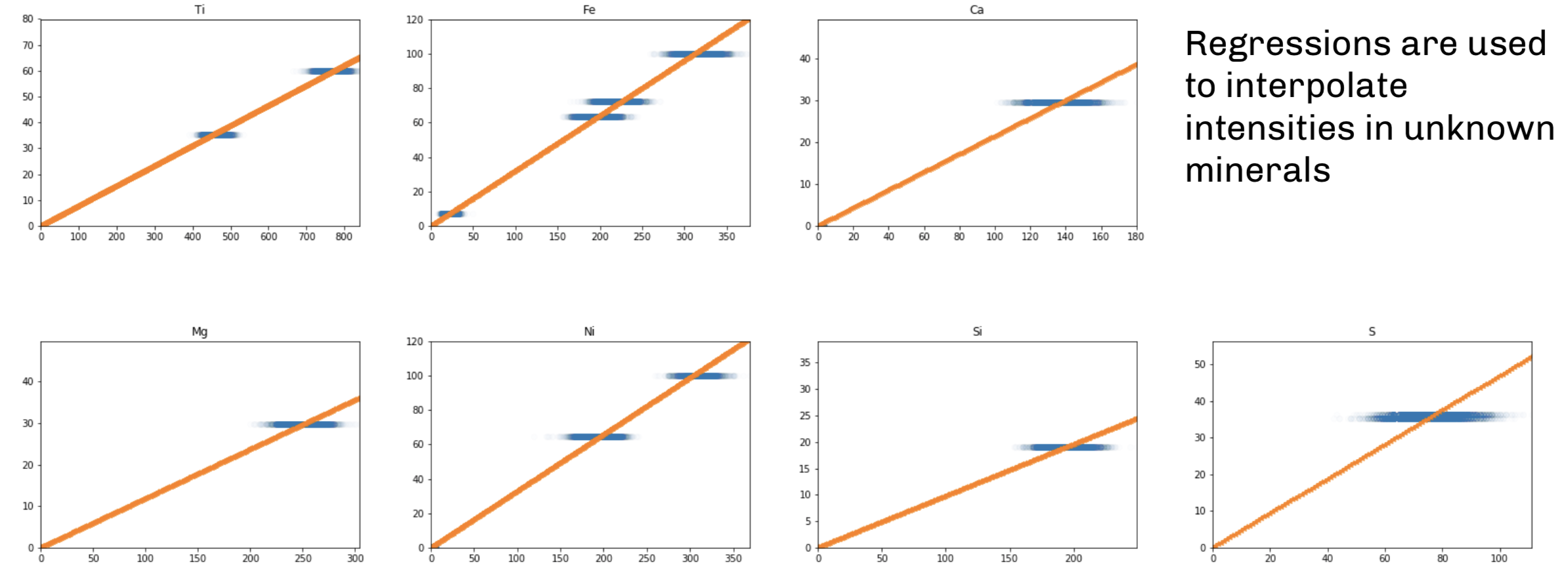
There is a linear relationship between pixel intensity and percent weight, so we used linear regression to find the slope of this relationship. We read in the .csv of pixel intensities for each element in the standards:

# read in the pixel intensities by element in the standard
mineral_standards = pd.read_csv('../../../static/mineralmapping/mineral_standards.csv')
print(mineral_standards.head())
##    Mg  Ni  Al  Fe   Ca  Cr  P  S   Ti  Si      mineral
## 0   0   0   0   0  171   0  4  0  459   0  CaTiO3std15
## 1   0   0   0   0  148   3  2  0  462   1  CaTiO3std15
## 2   0   2   0   0  141   6  3  0  455   2  CaTiO3std15
## 3   1   2   2   0  122   6  3  0  502   0  CaTiO3std15
## 4   0   0   0   0  138   5  5  0  457   1  CaTiO3std15

We modified the chemical formulas of each mineral using a dictionary by separating each element in the mineral with an “_” to make looping easier.

# create dictionary to standardize file names to chemical formulas
# needed to separate each element in the formula with an _ to make looping easier
mineral_dict = dict(zip(np.unique(mineral_standards['mineral']),
    ["Ca_Ti_O_3", "Fe_", "Fe_3O_4", "Fe_S_", "Ni_S_", "Ni_", "Ca_Fe_Mg_Mn_Ni_Si_", "Ti_O_2"]))
# use dictionary to change mineral columns to underscore format
weights['mineral'] = weights['mineral'].map(mineral_dict)
mineral_standards['mineral'] = mineral_standards['mineral'].map(mineral_dict)

Next we created a list of the elements accounted for in the standards and made an empty dataframe called coefs to fill with the coefficients of the relationship between pixel intensity and percent weight for each element:

# list of elements
# need to ignore the "mineral" column of the data
elements = [val for val in mineral_standards.columns if val != 'mineral']
coefs = pd.DataFrame(index = ['coeff'], columns = elements)

Linear regressions

Now we looped through the elements to create linear regressions of percent weight vs. pixel intensity based on the intensities in the standards. For these regressions, we forced the intercept to be zero because zero pixel intensity should imply zero percent weight.

# make a linear regression forcing the intercept to be zero
# since zero intensity should correspond to zero percent weight
lr = LinearRegression(fit_intercept = False)
# loop through elements to create linear regression of percent weight vs pixel intensity
# in the minerals in the standard
for element in elements:
    element_df = mineral_standards[mineral_standards['mineral'].str.contains(element + "_")]
    # if the element has no percent weights, skip it
    if element_df.empty:
        continue
    minerals = element_df['mineral'].unique()
    xis = np.empty(0)
    yis = np.empty(0)
    for mine in minerals:
        # get percent weights of the element in that mineral
        weight = weights[weights['mineral'] == mine][element]
        intensities = element_df[element_df['mineral'] == mine][element]
        xis = np.append(xis, np.array(intensities))
        yis = np.append(yis, np.repeat(weight, len(intensities)))

    xis, yis = xis.reshape(-1,1), yis.reshape(-1,1)
    # fit linear regression on percent weight vs intensity
    reg = lr.fit(xis,yis)
    xi_pred =  np.arange(0,900).reshape(-1,1)
    # create predictions for range of intensity values
    pred = reg.predict(xi_pred)
    reg.coef_
    # get the linear regression coefficient for each element
    coefs[element] = float(reg.coef_)
## array([[0.11859862]])
## <string>:26: DeprecationWarning: Conversion of an array with ndim > 0 to a scalar is deprecated, and will error in future. Ensure you extract a single element from your array before performing this operation. (Deprecated NumPy 1.25.)
## array([[0.32879587]])
## <string>:26: DeprecationWarning: Conversion of an array with ndim > 0 to a scalar is deprecated, and will error in future. Ensure you extract a single element from your array before performing this operation. (Deprecated NumPy 1.25.)
## array([[0.32008078]])
## <string>:26: DeprecationWarning: Conversion of an array with ndim > 0 to a scalar is deprecated, and will error in future. Ensure you extract a single element from your array before performing this operation. (Deprecated NumPy 1.25.)
## array([[0.21488656]])
## <string>:26: DeprecationWarning: Conversion of an array with ndim > 0 to a scalar is deprecated, and will error in future. Ensure you extract a single element from your array before performing this operation. (Deprecated NumPy 1.25.)
## array([[0.46922488]])
## <string>:26: DeprecationWarning: Conversion of an array with ndim > 0 to a scalar is deprecated, and will error in future. Ensure you extract a single element from your array before performing this operation. (Deprecated NumPy 1.25.)
## array([[0.07762688]])
## <string>:26: DeprecationWarning: Conversion of an array with ndim > 0 to a scalar is deprecated, and will error in future. Ensure you extract a single element from your array before performing this operation. (Deprecated NumPy 1.25.)
## array([[0.09790595]])
## <string>:26: DeprecationWarning: Conversion of an array with ndim > 0 to a scalar is deprecated, and will error in future. Ensure you extract a single element from your array before performing this operation. (Deprecated NumPy 1.25.)


# print the coefficients for each element
print(coefs)
##              Mg        Ni   Al        Fe  ...    P         S        Ti        Si
## coeff  0.118599  0.328796  NaN  0.320081  ...  NaN  0.469225  0.077627  0.097906
## 
## [1 rows x 10 columns]

Thus coefs contains the coeficient relating pixel intensity of an element to its percent weight in the mineral: for example, the percent weight of Mg in an mineral is equal to 0.118599 times its pixel intensity.

X-axes are pixel intensity and y-axes are percent weight of the element. Blue points indicate the pixel intensities of the element for a given percent weight based on a mineral in the standard. Orange points indicate the linear regression calculated above.

Calculate percent weights

Finally, we used these coefficients to calculate the predicted percent weights of each element in the two meteorites we were analyzing on a pixel-by-pixel basis. The code for this portion of the analysis is available in the latter end of this script. Note that for any pixel where the percent weight of an element was predicted to be higher than 100%, we set the percent weight to 100%. From these calculations, we ended up with the following files:

# read file of predicted percent weights for meteorite 1
df_obj1 = pd.read_csv('../../../static/mineralmapping/predicted_percentweight_obj1.csv')
df_obj1 = df_obj1.fillna(0)
df_obj1.drop('Unnamed: 0', axis = 1, inplace = True)
print(df_obj1.head())
##          Ca        Ti   Al   Cr  ...    P         Fe        Ni        Mg
## 0  8.595462  0.698642  0.0  0.0  ...  0.0  51.212925  0.986388  5.692734
## 1  4.512618  0.543388  0.0  0.0  ...  0.0  53.453490  1.972775  2.846367
## 2  2.578639  0.465761  0.0  0.0  ...  0.0  63.696075  3.287959  1.067388
## 3  2.148866  0.310508  0.0  0.0  ...  0.0  57.934621  3.945550  0.237197
## 4  1.719092  0.543388  0.0  0.0  ...  0.0  58.254702  3.616755  0.118599
## 
## [5 rows x 10 columns]


# read file of predicted percent weights for meteorite 2
df_obj2 = pd.read_csv('../../../static/mineralmapping/predicted_percentweight_obj2.csv')
df_obj2 = df_obj2.fillna(0)
df_obj2.drop('Unnamed: 0', axis = 1, inplace = True)
print(df_obj2.head())
##           Si    P   Cr   Al  ...        Ca        Mg        Ni         Fe
## 0  22.322556  0.0  0.0  0.0  ...  0.429773  1.304585  4.931938  14.403635
## 1  11.650808  0.0  0.0  0.0  ...  0.000000  0.355796  2.630367  43.530986
## 2   4.601580  0.0  0.0  0.0  ...  0.429773  0.000000  1.643979  54.093652
## 3   2.349743  0.0  0.0  0.0  ...  0.000000  0.000000  0.986388  57.294460
## 4   0.783248  0.0  0.0  0.0  ...  0.000000  0.000000  1.315183  48.972359
## 
## [5 rows x 10 columns]

Each row in these .csv files corresponds to a pixel in the original image. Each value gives the predicted percent weight of a given element in that pixel.

Up next

Now that we had converted pixel intensities to predicted percent weights, we were ready to use our clustering algorithm to identify potential minerals in the meteorite. Stay tuned for a future post showing how we used DBSCAN to accomplish this!